XRDMLread Examples
In this section you can find few demonstrations how to load and process data by the XRDMLread.
- Example no. 1 is a simple demonstration how to load a single scan using the XRDMLread function.
- Example no. 2 demonstrates visualisation of a two axes measurement data.
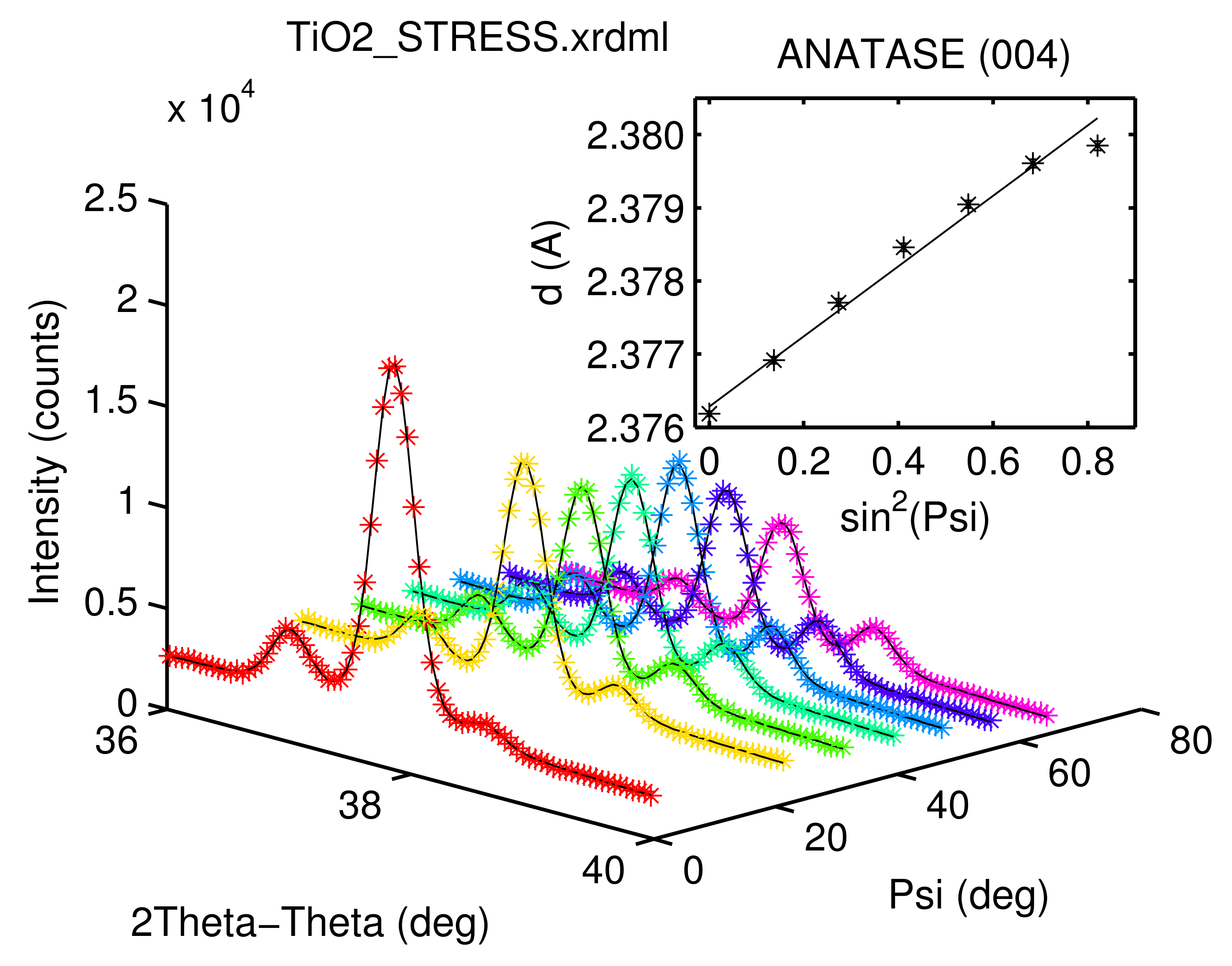
- Example no. 3 shows an application of the Sin2(Psi) method to three simultaneously measured neighbouring anatase lines of a Ti02 thin film sample.
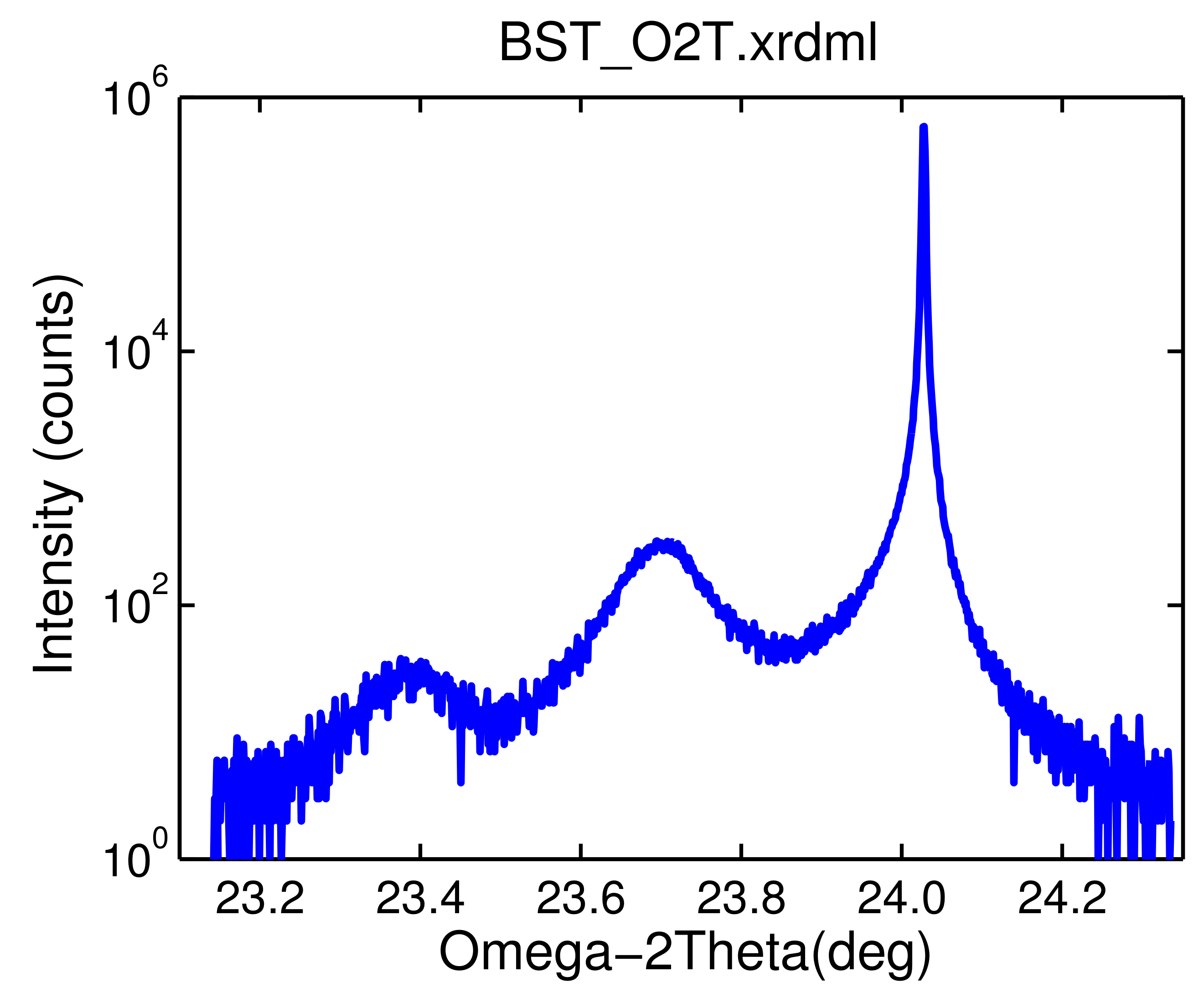
Example no. 1
is a simple demonstration how to load a single scan using the XRDMLread function.
% load XRDML data by a simple single command
d = XRDMLread('BST_O2T.xrdml') %#ok<NOPTS>

% plot data
figure

semilogy( d.x , round(d.data*d.time) )

box on

xlabel( [d.xlabel '(' d.xunit ')'] )
ylabel( 'Intensity (counts)' )

title( d.filename , 'Interpreter','none','FontName','Helvetica')
Download
- example1.m (src)
- BST_O2T.xrdml (data)
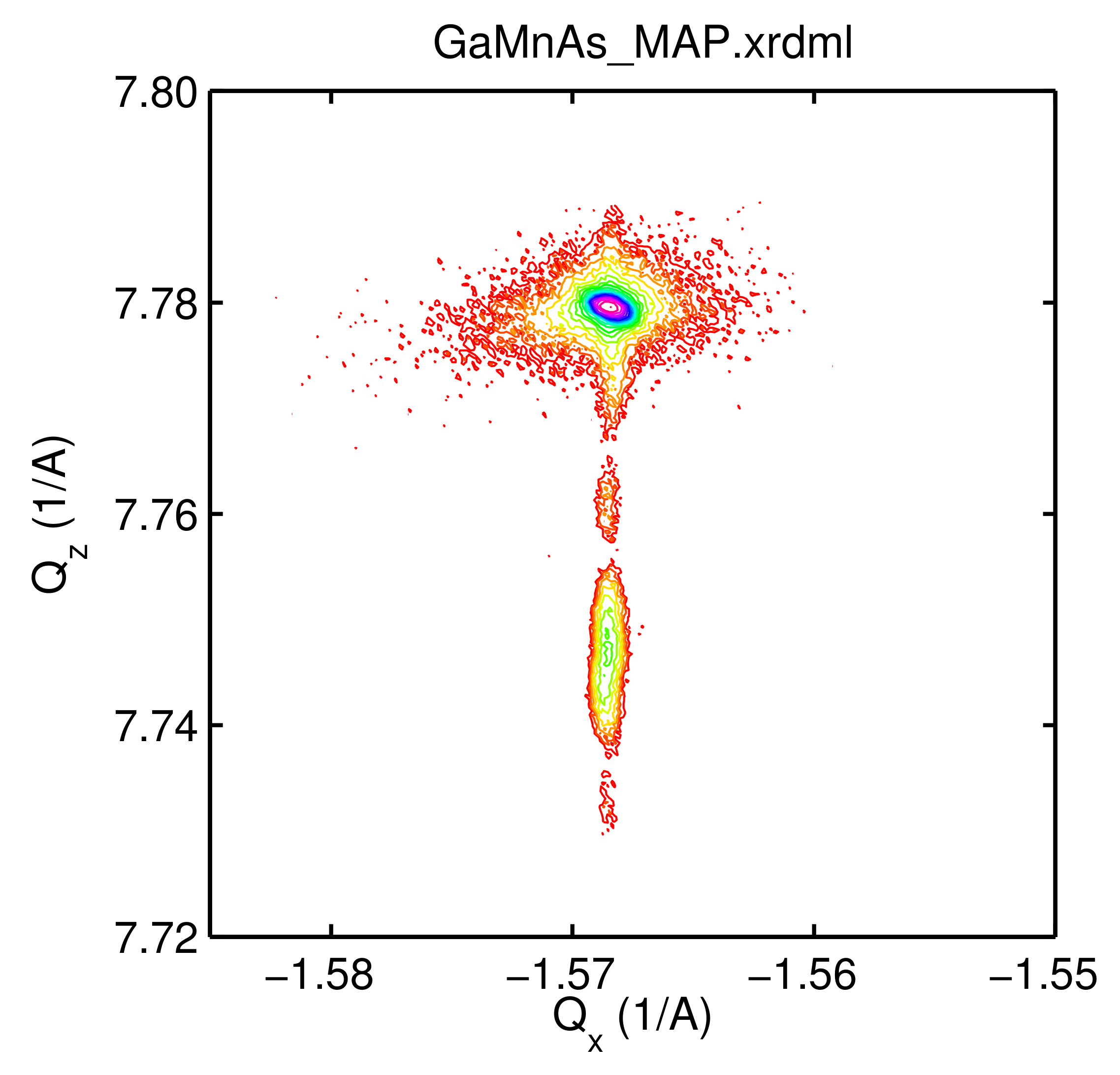
Example no. 2
demonstrates visualisation of a two axes measurement data.
d = XRDMLread('GaMnAs_MAP.xrdml') %#ok<NOPTS>

figure

% create an appropriate log scale
v = logspace( mean(d.data(d.data<5)) , log10(max(max(d.data))) , 21 );
col = hsv(21);

% calculate the contour matrix
C = contourc( d.Theta2(1,:) , d.Omega(:,1)-d.Theta2(:,1)/2 , ...
              d.data , v );

% transform contours coordinates into the Q-space
% and draw them
H = []; nn = 0; hold on
while nn+1<size(C,2)
    % extract data
    value = C(1,nn+1);
    level = find(v == value);
    dim = C(2,nn+1);
    ind = nn+1+(1:dim);
    x = C(1,ind); y = C(2,ind);
    % transformation
    Qx = 2*pi/d.Lambda*(-cos((x/2-y)*pi/180) + cos((x/2+y)*pi/180) );
    Qz = 2*pi/d.Lambda*( sin((x/2-y)*pi/180) + sin((x/2+y)*pi/180) );
    % draw line
    H(end+1) = line(Qx,Qz,'Color',col(level,:)); %#ok<SAGROW>
    % draw patch (Matlab)
    %H(end+1) = patch(Qx,Qz,col(level,:),'Line','none'); %#ok<SAGROW>
    % save data
    C(1,ind) = Qx;
    C(2,ind) = Qz;
    % increase index
    nn = nn+dim+1;
end

axis square
box on

xlabel('Q_x (1/A)')
ylabel('Q_z (1/A)')

title( d.filename ,'Interpreter','none','FontName','Helvetica')
Download
- example2.m (src)
- GaMnAs_MAP.xrdml (data)
Comment: In this example instead of a calculation of the contour plot in the non-equidistant Q-space points
the contours are rather calculated in the grid of measured points and then the transformed coordinates of the
equi-intensity lines are plotted manually.
Example no. 3
shows an application of the Sin2(Psi) method to three simultaneously measured neighbouring anatase lines of a Ti02 thin film sample.
d = XRDMLread('TiO2_STRESS.xrdml');

figure

hold on
col = hsv(length(d.Psi));
for k=1:length(d.Psi)
    plot3( d.Theta2(k,:) , repmat(d.Psi(k),1,size(d.data,2)) , ...
           round(d.data(k,:)*d.time), '*' , 'Color' , col(k,:) )
end
view(45,20)

xlabel( [d.xlabel ' (' d.xunit ')'] )
ylabel( [d.ylabel ' (' d.yunit ')'] )
zlabel( 'Intensity (counts)' )

title( d.filename , 'Interpreter','none','Interpreter','none','FontName','Helvetica')

% set global wavelength data for the pseudoVoigt function
global WAVELENGTHS
switch d.kType
case {'K-Alpha 1'}
    WAVELENGTHS = [1.0 0.0];
case {'K-Alpha'}
    WAVELENGTHS = [           1.0 (d.kAlpha1-d.Lambda)/d.Lambda ;
                    d.kAlphaRatio (d.kAlpha2-d.Lambda)/d.Lambda ];
otherwise
    warning('usedWavelength type not supported (using K-Alpha 1)')
    WAVELENGTHS = [1.0 0.0];
end

% add diffraction lines (anatase - database)
a0(1,:) = [56 36.95 0.2 0.5]; % (103)
a0(2,:) = [88 37.79 0.2 0.5]; % (004)
a0(3,:) = [36 38.57 0.2 0.5]; % (112)

% set refined lines parameters
Linda(1,:) = [1 1 1 0]; % (103)
Linda(2,:) = [1 1 1 1]; % (004)
Linda(3,:) = [1 1 1 0]; % (112)

results(1).hkl = [1 0 3];
results(2).hkl = [0 0 4];
results(3).hkl = [1 1 2];

% add linear background
b0 = [0.0 0.0];

% fit all scans
for k=1:length(d.Psi)
    x = d.Theta2(k,:);
    y = round(d.data(k,:)*d.time);
    w = 1./y;
    [a,b,da,db] = pseudoVoigtFit(x,y,w,a0,b0,[],Linda);
    yc = sum(pseudoVoigt(a,x),1) + polyval(b,x);
    for m=1:length(results)
        results(m).T2(k,1)  =  a(m,2);
        results(m).dT2(k,1) = da(m,2);
    end
    plot3( x , repmat(d.Psi(k),1,size(d.data,2)) , yc , 'k' )
end

% calc lattice planes distaces and their deviations
for m=1:length(results)
    th = results(m).T2*pi/360;
    results(m).d  = d.Lambda./2./sin(th);
    results(m).dd = cos(th)/d.Lambda.*results(m).d.^2.* ...
               results(m).dT2*pi/180;
end

% create sin^2(Psi) plots
x = sin(d.Psi*pi/180).^2;

for m=1:length(results)

    figure

    y = results(m).d; e = results(m).dd;
    [results(m).p,results(m).dp] = linfit(x,y,e);
    if ~exist('OCTAVE_VERSION'), %#ok<EXIST>
        errorbar( x , y , e , 'k*' ), hold on
    else
        plot( x , y , 'k*' ), hold on,
    end
    plot( x , results(m).p(1)*x+results(m).p(2) , 'k' )
    xlim( [-0.03, 0.9] )
    xlabel( 'sin^2(Psi)' ), ylabel ( 'd (A)' )
    str = sprintf('ANATASE (%d%d%d)', results(m).hkl);
    title( str )
end

% print results
for m=1:length(results)
    str = sprintf('   ANATASE DIFFRACTION LINE (%d%d%d)\n', ...
                  results(m).hkl);
    str = [ str sprintf('%14s%26s\n','Psi (deg)','2Theta (deg)') ];
    str = [ str sprintf('%14.4f%15.4f +/- %6.4f\n', ...
                 [d.Psi results(m).T2 results(m).dT2]' ) ];
    str = [ str sprintf('   D(HKL) VS. SIN^2(PSI)\n') ];
    str = [ str sprintf('%31s%23s\n','slope','intercept (A)') ];
    str = [ str sprintf('%15.4e +/- %11.4e %10.5f +/- %7.5f\n', ...
                 [results(m).p; results(m).dp]) ];
    disp(str)
end
Fitted peak positions and coefficients of the Sin2(Psi) linear regression are here (script output).
   ANATASE DIFFRACTION LINE (103)
     Psi (deg)              2Theta (deg)
        0.0000        37.0162 +/- 0.0026
       21.7200        37.0043 +/- 0.0032
       31.5500        36.9966 +/- 0.0031
       39.8600        36.9825 +/- 0.0030
       47.7300        36.9717 +/- 0.0029
       55.8300        36.9659 +/- 0.0029
       65.0000        36.9553 +/- 0.0033
   D(HKL) VS. SIN^2(PSI)
                          slope          intercept (A)
     4.7374e-03 +/-  2.5945e-04    2.42867 +/- 0.00012

   ANATASE DIFFRACTION LINE (004)
     Psi (deg)              2Theta (deg)
        0.0000        37.8637 +/- 0.0006
       21.7200        37.8516 +/- 0.0008
       31.5500        37.8386 +/- 0.0009
       39.8600        37.8261 +/- 0.0009
       47.7300        37.8164 +/- 0.0009
       55.8300        37.8072 +/- 0.0009
       65.0000        37.8032 +/- 0.0011
   D(HKL) VS. SIN^2(PSI)
                          slope          intercept (A)
     4.7994e-03 +/-  6.7711e-05    2.37628 +/- 0.00003

   ANATASE DIFFRACTION LINE (112)
     Psi (deg)              2Theta (deg)
        0.0000        38.6202 +/- 0.0072
       21.7200        38.6158 +/- 0.0045
       31.5500        38.5956 +/- 0.0038
       39.8600        38.5897 +/- 0.0032
       47.7300        38.5812 +/- 0.0026
       55.8300        38.5686 +/- 0.0025
       65.0000        38.5572 +/- 0.0027
   D(HKL) VS. SIN^2(PSI)
                          slope          intercept (A)
     4.5411e-03 +/-  3.1286e-04    2.33126 +/- 0.00018
Download
- example3.m (src)
- TiO2_STRESS.xrdml (data)
- peak-fitting-functions.zip
(compressed src)
- linfit.m (src)
Comment: Please note you need additional peak fitting functions and the linfit function to run this example.
See Add-ons section for more details.