Real structure and total powder pattern fitting. Program MSTRUCT
Radomír Kužel1, Zdeněk Matěj2, Milan Dopita1
1Charles University, Faculty of Mathematics and Physics, Ke Karlovu 5, 121 16 Praha 2
2MAX IV Laboratory, Lund University, Lund, Sweden
kuzel@karlov.mff.cuni.cz
Real structure and classical XRD line profile analysis
The term “real structure” is often used but not clearly defined. We have discussed this in relation to a short course on real structure of materials included in Struktura 2009 in Hluboká nad Vltavou [1]. In XRD, real structure is related mainly to lattice defects in atomistic scale, and in a larger scale to size, shape and distribution (possibly preferred orientation) of grains (or crystallites – coherently diffracting domains) and also their interactions (residual stress). The fields of texture analysis and residual stress analysis have been developed and for the X-ray diffraction they consist in measurement of integrated intensities of selected diffraction peaks hkl in dependence on the angle of the corresponding lattice plane with respect to the surface and analysis of peak positions in the same dependence, respectively. The analysis of lattice defects can be done for example by careful study of diffuse scattering which is usually possible only for single crystals or the so-called XRD line profile analysis. The latter procedure was also described briefly in [1].
XRD line profile analysis can be done directly on individual well-separated diffraction peaks by determination of some relevant parameters as for example FWHM (full-width-at-half-of-maximum), integral breadth, moments – mainly the second moment variance and Fourier coefficients (FC). These parameters can be subsequently analyzed and some physical characteristics like crystallite size and microstrain are determined. However, in this procedure, for laboratory data Ka2 component must be separated either before the determination of parameters or after that which was done in the past. Then it must be considered that the measured profile is convolution of physical profile with the instrumental one containing the influence of geometry and optics of the instrument and broadening of spectral lines. Therefore, some deconvolution or correction must be performed, unless the difference between the instrumental and physical broadening is large like for example in really nanocrystalline materials (with the crystallites e.g. below 10 nm). Some of the methods were described for example by Klug and Alexander [2]. For approximative method using just line widths there are a few simple methods of correction of instrumental broadening. Famous Warren-Averbach (WA) [3] analysis consists of several steps. Typically, the FC of several diffraction profiles of the standard sample are determined as coefficients corresponding to the instrumental profile, then the FC for diffraction peaks of several reflection orders of analyzed sample are calculated and for example the Stokes method [see 3] (with a benefit of not necessary Ka2 elimination) is applied and the finally obtained FC of the physical profile are analyzed by the WA method. This is a several-steps procedure with some critical points, mainly the deconvolution of noisy and finite profiles.
Rietveld analysis
In practice, we must work quite often with heavily overlapped profiles, sometimes even for one phase. In this case, peaks are usually fitted with some suitable phenomenological peak-shape functions, mainly the Pearson VII, pseudo-Voigt or Voigt functions, describing quite well profiles of individual components. Then, basically, we could proceed as in the previous case. Of course, by such fitting, some profile features can be masked. Principle difference between the so-called size and strain broadening is its different behavior in reciprocal space, the former being constant and the latter proportional to the diffraction vector magnitude, respectively. Significant anisotropy (hkl dependence) can be caused by anisotropic crystallite shape for the former effect and for example dislocation type in the latter case, respectively.
In sixties, the Rietveld method appeared [e.g. 4] which later has become extremely popular. The idea of the method is to describe whole powder diffraction pattern with a suitable function containing everything relevant in some, if possible analytical, function with free parameters to be determined. Then, in principle, all required characteristics could be get in a few iterations. Of course, it is often not so simple. The first aim was to apply the analysis for structure refinement since the integrated intensities are primarily related to the structure factors, that means also atomic positions. Peak positions are related to the lattice parameters. Quite quickly the Rietveld method was also used for the phase analysis. However, since all relevant effects must be included in the procedure also parameters related to real structure were considered, usually in some more or less phenomenological way. They described texture, size and strain line broadening in some cases also residual stress and nowadays they are including also anisotropic effects. Probably, the most popular classical Rietveld type programs are FULLPROF by Juan Rodriguez-Carvajal [5] and GSAS by Bob von Dreele [6]. There are also others (see [7, not updated] for available Rietveld software) like BGMN [8] by Joerg Bergmann, BRASS [9] and, of course, there is also powder pattern fitting in famous Jana2006 [10]. There are also commercial Rietveld or multiple purpose programs like TOPAS (Bruker), High-Score (Panalytical) and others.
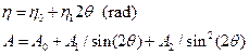
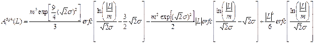
Most of these programs use the so-called Cagliotti polynomial
![]() (1)
(1)
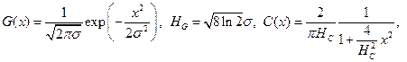
for the description of angle-dependence of instrumental XRD line broadening. In case, the corresponding profile function used is the pseudo-Voigt (weighted sum of Gauss and Cauchy functions), we can introduce also angle dependence of Cauchy-Gauss mixing parameter h and possibly asymmetry A as follows
 (2)
(2)
The parameters U, V, W, h0, h1, A0, A1, and A2 are determined by the fitting of standard diffraction pattern measured on the same instrumental arrangement as the one used for the measurement of the investigated samples. These relations are often extended and used also for the analysis of the physical broadening, in last versions of the above programs in very flexible and more general way.
It seems that the most comprehensive description of instrumental effects it is the so-called fundamental parameters approach consisting in calculation of all instrumental and spectral components. This was introduced mainly by R.W. Cheary and it is used in TOPAS and also in Jana now.
The use of the Voigt or more pseudo-Voigt functions is preferred now to the Pearson VII. The Cauchy (Lorentz) and Gauss functions can be expressed as follows
 (3)
(3)
Where HC and HG are FWHMs of the Cauchy and Gauss components, respectively.
Extension of polynomial (1) is made slightly differently in FULLPROF, GSAS and Jana. In Jana, similarly to GSAS the Gauss FWHM is written as [11]
![]() (4)
(4)
where the fourth term is the Scherrer coefficient for Gauss broadening.
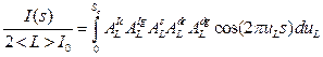
The Cauchy FWM is composed of five terms:
![]() (5)
(5)
The X terms accounts for Lorentzian Scherrer particle broadening and stands for isotropic and anisotropic part, respectively. j is the angle between the diffraction vector and the broadening direction. The Y terms describe strain broadening. The last term stands for the Stephen's strain anisotropy, where the anisotropic strain is described by a symmetrical 4th order tensor [12] and this contribution to FWHM is
![]() (6)
(6)
GSAS [13, more recent 14] offers several functions for time-of-flight and for XRD and constant wavelength neutron diffraction and XRD. Basically, some of them are similar as the above functions used in Jana. They can include possible asymmetry, anisotropy and one of them also effect of macroscopic strain.
FULLPROF uses equations quite similar as (4-5).
![]() (7)
(7)
![]() (8)
(8)
where D and F functions have different expressions depending on the particular model of size and strain broadening. The parameter x is mixing coefficient to mimic Cauchy contribution to strains. The metric parameters ai are considered as stochastic variables with Gaussian distribution characterized by the mean value and the variance-covariance matrix [15]. The anisotropic strain broadening is modelled using a quartic form in reciprocal space. The Stephens approach can be used as well. FULLPROF offers different models for size (e.g. needle-like domains) and strain (with different symmetries of strain and lattice), and also possibility to define some reflection families (for specific hkl broadened or unbroadened) which can simulate the effect of stacking faults. The same is possible to introduce in GSAS. The anisotropic crystallite shape is modelled with a linear combination of spherical harmonic functions ylmp normalized according to M. Järvinen [16]. The size contribution to integral breadth b is
![]() (9)
(9)
The arguments are the polar angles of the vector h with respect to the Cartesian crystallographic frame.
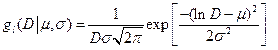
Total powder diffraction pattern modelling and fitting
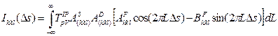
Another way came from the groups primarily dealing with the real structure. The first one was Charles Houska [17, 18]. As he realized the mentioned above problems of several-steps WA analysis, he tried to describe the whole individual profile by physical function. The profile function I(s = 2 sin q/l) was expressed in terms of the Fourier coefficients of individual components including instrumental ones (replacing in such a way deconvolution with convolution, the way dominating nowadays). The physical FC included two parameters related to the crystallite size effect and two more or less phenomenological microstrain parameters as follows
 (10)
(10)
where AIc and AIg correspond to the Cauchy and Gauss component of the Voigt function used for approximation of the instrumental profile, <L> is mean crystallite size in the measured direction uL = L/<L>. Integration limit Sc is dependent on the variation coefficient of crystallite size distribution Vc, Sc = 1+Ö3Vc. The size coefficients As can be expressed as the third-order polynomial of u, and there are two types of strain coefficients
![]() (11)
(11)
![]()
with the so-called uniform (eU) and nonuniform strain (eD) related to the mean-square strain as
![]() (12)
(12)
The relation is empiric based on many observed cases. The functions were simultaneously fitted to several reflection orders or neglecting anisotropy just to a few diffraction profiles with different hkl. The method was later extended with stacking faults. Examples are also shown in [19]. There is no software currently available for the method.
Later, Rietveld-type programs focused on real structure have been developed by Matteo Leoni and Paolo Scardi in Trento, Pm2k [20-23] and Gábor Ribárik in Budapest, CMWPFIT [24-25]. Separately, also quite well-known system MAUD was developed by Luca Lutterotti [26-28]. Each of the programs has some features which are common and also some which are unique. Since we have not been fully satisfied with any of these, we have been developing our own system MSTRUCT [29-32] written by Zdeněk Matěj as extended FOX system [33] based on Crystal Objects library. All the above programs are freely available, some of them require registration.
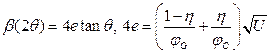
CMWPFIT, Pm2k and MSTRUCT are basically working with similar algorithms for the description of size and dislocation broadening
Total formula for peak profile is like this, similar as description by Houska (9)
 (13)
(13)
with instrumental Fourier coefficients T, size, strain and stacking fault FTs AS, AD and AF, respectively.
Physical effects can be conveniently modelled in real space (Fourier coefficients). The size broadening effect is described by the model function for log-normally distributed spherical crystallites with two parameters to be refined—median of crystallite size and variance of the distribution or alternatively by the distribution histogram.
The expression for the size distribution can look as follows [e.g. 24]
(14)
Very popular and often also realistic is log-normal size (D) distribution with two parameters m and s.
 (15)
(15)
The strain broadening can be described by the dislocation model including three parameters—dislocation density, dislocation-correlation parameter, cut-off radius, and dislocation types - fraction of edge dislocations. Assuming probable dislocation types the contrast factors c can be calculated in specific cases. The strain Fourier coefficients can be written as
![]() (16)
(16)
![]() where
b is the Burgers vector magnitude, r
is the dislocation density, d* the interplanar spacing of the first
order reflection, Rc cut-off radius (dislocation-correlation
parameter) and f* complicated but known van Berkum or Wilkens function.
For cubic materials, the orientaion factor can be written as follows
where
b is the Burgers vector magnitude, r
is the dislocation density, d* the interplanar spacing of the first
order reflection, Rc cut-off radius (dislocation-correlation
parameter) and f* complicated but known van Berkum or Wilkens function.
For cubic materials, the orientaion factor can be written as follows
![]() (17)
(17)
with two parameters A, B to be fitted or calculate.
CMWPFIT is focused on the analysis of some microstructural parameters for cubic or hexagonal materials. The whole measured powder diffraction pattern is fitted by the sum of a background function and ab-initio theoretical functions for size and strain broadening. In the calculation of the theoretical functions it is assumed that the crystallites have lognormal size distribution and the strain is caused by dislocations. Strain and size anisotropies are taken into account by the dislocation contrast factors and the ellipticity of crystallites. The fitting procedure provides the median and the variance of the size distribution and the ellipticity of crystallites, and the density and arrangement of dislocations. Instrumental correction is convoluted. There are no other effects included. The program is working on-line.
Pm2k [23] has been designed with modularity and expansibility in mind. Three main entities can be identified in the program: kernel, plug-ins and user interface. The kernel is performing nonlinear least squares minimisation. Plug-ins are compiled independently as dynamic loading libraries and linked to the kernel at runtime. Users can easily implement their own models into the kernel. There are quite a lot of interesting features included (implemented as plugins)
Instrumental broadening: Rietveld-Caglioti formula.
Size broadening: histogram model for size distribution (sphere, cube, tetrahedron, octahedron, ellipsoid, hexagonal prism, cylinder, harmonics), analytical model for size distribution (delta, lognormal, gamma, generalised gamma, York distributions of sphere, cube, tetrahedron, octahedron, ellipsoid, hexagonal prism, cylinder, harmonics).
Strain broadening: dislocations (fcc,bcc,hcp) using the simplified and full Wilkens models o dislocations (all symmetries) using harmonics invariant or Green function. Houska-like models (Houska, Adler-Houska, modified Houska)
Stacking faults for fcc, bcc and hcp o correlation probability, antiphase boundaries. Grain surface relaxation effect
Additional broadening models: grain-dependent lattice parameter variation, broadening due to stoichiometry fluctuations.
The programs runs via interface but basically runs on the base of input and output file.
MAUD is probably the most complex program available for the analysis of real structure but it does not include dislocation models. Regular schools on the software are organized in France. There is no manual but several tutorials available. The program is written in Java and controlled by a GUI with many optimization algorithms available and can work with X-ray, synchrotron, neutron, TOF and electron diffraction data. It can simultaneously fit several different spectra, work with the data from 2D detectors, with fluorescence data. It can fit reflectivity curves and it can also make complete texture and residual stress analysis using part or full spectra. The program is well-adopted for the analysis of thin film and multilayers and of course microstructure analysis (size-strain, anisotropy, planar defects, turbostratic disorder and distributions) is included.
MSTRUCT program is a subject of the course at this meeting and during last years different features have been included affecting different XRD line profile parameters as described for example in [30].
Peak positions are determined by variable unit-cell parameters and zero-shift error. Specimen displacement error is not considered for the parallel-beam geometry but included for symmetrical q-2q scans. For low angles of incidence close to the angle of total reflection, which are required for very thin films, mainly below 1°, refraction correction must be included. Residual stress can influence the peak positions. Peak shifts then can also be anisotropic. The effect of residual stress in the current version of MSTRUCT is included for simple symmetrical biaxial stress in the plane of a sample surface and can be hkl dependent. X-ray elastic constants s1(hkl), s2(hkl) are calculated in two extreme models of grain interactions—Reuss and Voigt. In the case of lower symmetry, they can be conveniently calculated according to [34-36], and then two refinable parameters i.e., residual stress and fraction of the Voigt-Reuss models appear.
Peak intensities are calculated by the ObjCryst library from a known crystal structure. The structural parameters can be varied when necessary. However, they are used as constraints for the peak positions and intensities. The effects of absorption and texture correction in a thin film can be included. In general, the texture correction can be obtained from a known model of the ODF after appropriate integration over all crystallites with diffracting (hkl) planes perpendicular to the direction of the measured diffraction vectors both for asymmetric and symmetric scans. In principle any type of the ODF function can be supplied to the algorithm and used for texture correction, but only a simple model using the Gaussian distribution of crystallites and possible inclinations of texture with respect to the sample normal is included.
Peak profiles are given by numerical convolution of a known instrumental function and physical profiles including several refinable parameters. Size and dislocation-induced strain broadening are described above. For some cases, phenomenological microstrain broadening can be useful. For this case, the peak broadening is modeled by the pV function and its FWHM angular dependence is given by the Cagliotti polynomial containing only the quadratic term U. This means that the FWHM in reciprocal space units is linearly increasing with the diffraction vector magnitude. The shape factor of the pV function common for all hkl diffraction peaks can also be refined. Then relations for microstrain e can be used.
 (18)
(18)
where jG = 2(ln(2)/p)1/2 and jC = 2/p are the Gauss and Cauchy shape parameters, respectively
Anisotropic size broadening model was introduced
in MSTRUCT. A model of rods and platelets like crystallites were also
complemented with quite common model of ellipsoidal shape.
If appropriate specific model is unknown a possibility of arbitrary hkl
dependent multiplication factors for peak intensities and also peak shifts can
be introduced.
New non-standard models in MSTRUCT were described in a lecture at Struktura 2017. These are for example: stacking faults on prismatic planes in WC, Warren-Bodenstein model for turbostratic nanoparticles, configuration model for description of bimodal microstructure, unconventional analysis of nanocrystalline and amorphous like materials [37].
1. R. Kužel, Materials Structure, vol. 2a (2009) k71-k77. http://www.xray.cz/ms/bul2009-2a/courses.pdf
2. H. P. Klug, L. E. Alexander, X-ray Diffraction Procedures for Polycrystalline and Amorphous Materials. NewYork, 1974.
3. B. E. Warren.: X-Ray Diffraction. Addison-Wesley. Reading. 1969.
4. The Rietveld Method, ed. R. A. Young, IUCr series, Monographs on Crystallography (1995).
5. https://www.ill.eu/sites/fullprof/
6. https://subversion.xray.aps.anl.gov/trac/pyGSAS
7. http://www.ccp14.ac.uk/solution/rietveld_software/
8. http://www.bgmn.de/
9. http://www.brass.uni-bremen.de/
10. http://jana.fzu.cz/
11. http://jana.fzu.cz/doc/powder_parameters.pdf
12. P. Stephens, J. Appl. Cryst. 32 (1989) 281-289 (1999).
13. http://www.ccp14.ac.uk/ccp/ccp14/ftp-mirror/gsas/public/gsas/manual/GSASManual.pdf (p. 156-165).
14. Toby, B. H., & Von Dreele, R. B. J. Appl. Cryst., 46(2) (2013) 544-549.
15. FULLPROF manual, p. 20-31. (installation or https://www.psi.ch/sinq/dmc/ManualsEN/fullprof.pdf)
16. M. Jarvinen, J. Appl. Cryst. 26 (1993) 527.
17. T. Adler, C. R. Houska, J. Appl. Phys. 17 (1979) 3282-3287.
18. C. R. Houska, T. M. Smith, J. Appl. Phys. 52(2) (1981) 748-754.
19. Microstructure Analysis from Diffraction, edited by R. L. Snyder, H. J. Bunge, and J. Fiala, International Union of Crystallography, 1999.
20. P. Scardi, M. Leoni, in Diffraction Analysis of the Microstructure of Materials (Eds. E. J. Mittemeijer, P. Scardi) pp.51-92. Springer. Berlin. Heidelberg. 2003.
21. P. Scardi, M. Leoni, Acta Cryst. A58 (2002) 190-200.
22. P. Scardi, M. Leoni Y. H. Dong, Eur. Phys. J. B18 (2000) 23-30.
23. M. Leoni, T. Confente, P. Scardi, Z Kristallogr., Suppl. 23 (2006) 249-254.
24. G. Ribárik, T. Ungár, J. Gubicza, J. Appl. Cryst. 34 (2001) 669-676.
25. http://csendes.elte.hu/cmwp/
26. http://maud.radiographema.eu/
27. L. Lutterotti, Nuclear Inst. and Methods in Physics Research, B268, 334-340, 2010.
28. L. Lutterotti, M. Bortolotti, G. Ischia, I. Lonardelli and H.-R. Wenk, Z. Kristallogr., Suppl. 26, 125-130, 2007.
29. http://www.xray.cz/mstruct
30. Z. Matěj, R. Kužel and L. Nichtová, Powder Diffraction, 25 S2 (2010) p. 125-131. doi: 10.1154/1.3392371.
31. Z. Matěj, A. Kadlecová, M. Janeček, L. Matějová, M. Dopita and R. Kužel, Powder Diffraction, 29 S2 (2014), p. S35-S41. doi: 10.1017/S0885715614000852.
32. L. Matějová, M. Dopita and R. Kužel, Refining bimodal microstructure of materials with MSTRUCT, Powder Diffraction 29 S2 (2014), p. S35-S41. doi: 10.1017/S0885715614000852.
33. V. Favre-Nicolin & R. Cerny, J. Appl. Cryst. 35 (2002), 734. doi: 10.1107/S00218898020
34. N. C. Popa, J. Appl. Cryst, 33 (2000) 103–107.
35. N. C. Popa and D. Balzar, J. Appl. Cryst. 34 (2001) 187–195.
36. Behnken, H. and Hauk, V. 1986. “Berechnung der rontgenographishen elastizitatskonstabten REK des vielkristalls aus den einkristalldaten fur beliebige kristallsymmetrie,” Z. Metallkd. 77, 620–626.
37. Z. Matěj, M. Dopita, J. Endres, Materials Structure, vol. 24 (2017) 18-20
The work is supported by the “NanoCent” Project No. CZ.02.1.01/0.0/0.0/15_003/0000485, financed by ERDF.