Real structure of polycrystalline materials
Short
course
R. Kužel
Faculty of Mathematics and Physics,
Charles University in Prague, Ke Karlovu
5, 121 16 Prague 2
kuzel@karlov.mff.cuni.cz
1. Introduction
During
last decades, it has been shown many times that properties of materials are not
determined only by phase composition and crystal structure but very often the
so-called real structure plays an important role. What should we imagine under
this name – real structure of crystalline
materials? There is no clear definition but in the most general view it is
any violation of ideal translation periodicity of atoms. If we consider a
single crystal, this is already its finite dimension, the surface that breaks the periodicity and may lead to creation of a
new 2D structure. This is not usually understood as real structure, though, but
rather it belongs to a large and important branch of science – surface
crystallography, surface physics and surface chemistry (see also [1, 2]).
Other
deviations from ideal atomic positions are thermal
lattice vibrations. They can be studied by several methods, in particular,
by neutron scattering and they are considered in XRD in terms of the so-called
Debye-Waller factors. The factors are sometimes approximated by a mean
isotropic DW factor common for all atoms but exactly they should be included in
the product with individual atomic scattering factors and even better in
anisotropic form and perhaps also including anharmonic
contributions. However, the vibrations are not meant under the name “real
structure” either.
For single crystal, the term is closely connected to the lattice defects. There are many types of lattice defects – point, line, plane (2D) or volume (3D). Some of them are schematically shown in Fig. 1. There are several methods for study of point defects like differential thermal expansion, positron annihilation (e.g. [3]), resistivity, specific heat and, of course, also imaging methods with high resolution like HRTEM, STM, AFM, FIM. The line defects – dislocations and higher dimension defects can be traditionally studied by TEM. In the framework of kinematical theory of diffraction the lattice defects can be divided into two kinds according to their influence on the diffraction pattern. This has been derived and suggested by Krivoglaz [4]. The lattice defects of the first kind are the defects with rapidly decreasing field and lead to the reduction of integrated intensity (static Debye-Waller factor), shift of the Bragg peaks and appearance of diffuse scattering. The defects of the second kind with slowly decreasing (1/r) displacement field, destroy the Bragg sharp peak and only concentrated diffuse scattering can be observed as the broadened quasiline – the lattice defects of the second kind. Point defects, their clusters, precipitates and small dislocation loops belong to the former while dislocations to the latter type. The type of displacement field plays the most decisive role for the classification of the defects. This is based on the physical nature of the defects and it has been derived for their random distribution. However, the situation is more complicated in practice. Only a few models for non-random defect distribution have been developed and used so far.
Since different effects are produced by both lattice defect types, different X-ray methods are applied for their investigation. The studies of defects of the first kind are mostly restricted to single crystals and consist in simultaneous measurement of lattice parameters, static Debye-Waller factors and whole maps of diffuse scattering. The diffuse scattering is probably the best source of information on point defects and their clusters since it is very sensitive to the type, arrangement and orientation of the defects and often even a simple comparison of experimental and simulated contour plots can be very helpful. The study of defects of the second kind can also be done for polycrystalline samples and it consists in the XRD line profile analysis. The classification of the lattice defects from the point of view of XRD should not be mixed with the classification of stresses. In this connection, all the distortions by point and line defects belong to the so-called 3rd kind stresses.
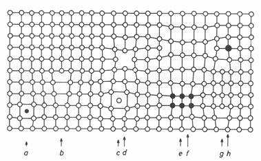
Figure 1. Picture of different types of lattice defects - a) Interstitial impurity atom, b) Edge dislocation, c) Self interstitial atom, d) Vacancy, e) Precipitate of impurity atoms, f) Vacancy type dislocation loop, g) Interstitial type dislocation loop, h) Substitutional impurity atom ([3])
In addition to the above effects, real structure of polycrystalline materials includes also larger scale effects. This is distribution of size and orientation of individual grains and also their interactions, stresses. The maps of grains are nowadays studied more and more by the EBSD (Electron backscattered diffraction) [5], very powerful method which however, is quite critical to sample preparation. 3D maps can also be constructed from XRD measurements of individual grains by synchrotron radiation [6, 7] (beamlines in APS and ESRF). In X-ray laboratory, such studies are always connected with measurements of diffracted intensities of individual (hkl) planes in dependence on the orientation of the plane with respect to the specimen coordinate system – for texture investigation and/or diffraction peak positions (lattice spacing) in the same dependence – for residual stress measurement.
The investigation of real structure by diffraction methods is of great interest nowadays and still many unresolved problems. Several books appeared on the topics [e.g. 8, 9].
Figure 2a. Preferred grain orientation may cause significant changes of integrated intensities of hkl peaks in symmetric scans and their variation with inclination of corresponding planes with respect to the specimen surface.
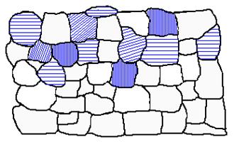
Figure 2b. Residual stress results in variation of interplanar spacing with inclination of the planes with respect to the specimen surface.
2. XRD line profile analysis
XRD line profile analysis is used for the determination of microstrain and/or dislocation density, crystallite size
and sometimes also other defects like stacking faults. All these factors cause XRD line broadening.
There are number of ways how they are included in present Rietveld
programs. In most cases, though, phenomenological models are used and their
main aim is to correct the pattern for these defects in order to refine crystal
structure or make phase analysis and no to determine the above parameters.
2.1 Characterization of individual profiles
The diffraction line profile can be expressed as the dependence of
intensity (e.g. in cps – counts per second) on the diffraction angle 2q or on the
diffraction vector magnitude (s = 2 sin Q/l). The profile can be characterized by several parameters related directly
to some structural and/or microstructural parameters:
peak positions ® lattice parameters, lattice
geometry, lattice defects, residual stress
integrated intensities ® atomic structure, texture,
lattice vibrations
peak widths ® internal strains, coherent domain
size, lattice defects
peak shape ® distribution of lattice defects
and domains
Any of these characteristics can be determined from a single powder
diffraction pattern for each phase separately. For the analysis of line
broadening several parameters can be used:
FWHM (half-width, full width at
half of peak maximum)
Integral breadth (b) – integrated intensity I over peak height in the finite
range s1 to s2
 (1)
(1)
The ratio of this
two widths is sensitive to profile shape.
Moments
 (2)
(2)
Fourier coefficients
 (3)
(3)
(Ds = s2 – s1 is the integration range, L is a variable in the direct space )
These parameters can be determined by about three different methods:
- Direct analysis of isolated lines
- Fitting of suitable analytic functions (Pearson, pseudo-Voigt,
Voigt) to the groups of diffraction profiles
- Total
pattern fitting either with or without structural constraints
The first method can include background separation, smoothing, Ka2 elimination and
determination of the above parameters. This was applied already in classical
profile analysis [10, 11]. The a2 elimination was
based mainly on Rachinger algorithm [12], in improved way for example in [13].
Different analytical functions were applied (comparison in [14, 15], other
functions can be found in [16, 17]) for the second and/or third method.
2.2 Instrumental broadening
Unfortunately, similarly to other physical
methods we cannot measure pure physical effect (broadening) but this is smeared
out by the instrument. This can be described as mathematical convolution.
Measured profile is usually denoted as h,
instrumental as g and physical as f. Then h = f ٭g (or ![]() ) and f profile
must be obtained by the deconvolution. There are a
number of deconvolution methods but always with a
problem of mathematically incorrect procedure since the functions are not known
in infinite range and there is also experimental noise in the data [18]. The
problems can be reduced by the so-called regularization but always there should
be an effort to minimize instrumental broadening, i.e. to increase resolution.
Of course, it goes always on the cost of intensity. If we can reduce the
influence of g, then depending on a
problem (ratio of physical to the instrumental broadening) the instrumental
broadening can either be completely neglected or on the other hand finer
physical effects can be measured (larger crystallites, lower defect densities).
Conventional powder diffraction (parafocusing
Bragg-Brentano) can have quite good resolution, in particular, if the primary a1 monochromator is used. The problem is in the
analysis of thin films when the symmetric scan is often inconvenient because of
larger penetration depth and for asymmetric scans parallel beam geometry is
preferred (mirrors, parallel plate collimators). Depending on the used parallel
plate collimator, this arrangement has usually rather poor resolution (about
three times worse than Bragg-Brentano). The resolution can be improved by
different ways - for example double-mirror setup, channel-cut monochromator, hybride monochromator, crystal analyzers etc. but with sometimes
drastically reduced intensity not very usable with conventional X-ray sources.
The methods of deconvolution can be divided into
several groups according to characterization of profiles – full profile deconvolution, Stokes correction of Fourier transform
(Fourier transform of the convolution is a product of Fourier transforms),
approximate methods of integral breadths (Voigt function) or simple subtraction
of the second moments (variances). Another problem can be the determination of g profile. In most cases, standard
sample with negligible physical broadening is measured under the same
conditions as the investigated sample. NIST was selling LaB6
standard for line broadening but this is out of stock now. Optimal standard
should be the same material as the one investigated mainly because of
absorption. This may be achieved by annealing of suitable sample but the
results are uncertain. Therefore each laboratory should select suitable
standards according to its experience. The second way may be to calculate g from known geometrical parts of the
instrument (slits) and spectral lines. This has been suggested by R. W. Cheary [19] and it is used in commercial software TOPAZ (Bruker). The software uses also another popular way – to
replace ill-defined deconvolution by the fitting of
the pattern with a convolution of the known instrumental profile and physical
or phenomenological function of several refineable
parameters.
) and f profile
must be obtained by the deconvolution. There are a
number of deconvolution methods but always with a
problem of mathematically incorrect procedure since the functions are not known
in infinite range and there is also experimental noise in the data [18]. The
problems can be reduced by the so-called regularization but always there should
be an effort to minimize instrumental broadening, i.e. to increase resolution.
Of course, it goes always on the cost of intensity. If we can reduce the
influence of g, then depending on a
problem (ratio of physical to the instrumental broadening) the instrumental
broadening can either be completely neglected or on the other hand finer
physical effects can be measured (larger crystallites, lower defect densities).
Conventional powder diffraction (parafocusing
Bragg-Brentano) can have quite good resolution, in particular, if the primary a1 monochromator is used. The problem is in the
analysis of thin films when the symmetric scan is often inconvenient because of
larger penetration depth and for asymmetric scans parallel beam geometry is
preferred (mirrors, parallel plate collimators). Depending on the used parallel
plate collimator, this arrangement has usually rather poor resolution (about
three times worse than Bragg-Brentano). The resolution can be improved by
different ways - for example double-mirror setup, channel-cut monochromator, hybride monochromator, crystal analyzers etc. but with sometimes
drastically reduced intensity not very usable with conventional X-ray sources.
The methods of deconvolution can be divided into
several groups according to characterization of profiles – full profile deconvolution, Stokes correction of Fourier transform
(Fourier transform of the convolution is a product of Fourier transforms),
approximate methods of integral breadths (Voigt function) or simple subtraction
of the second moments (variances). Another problem can be the determination of g profile. In most cases, standard
sample with negligible physical broadening is measured under the same
conditions as the investigated sample. NIST was selling LaB6
standard for line broadening but this is out of stock now. Optimal standard
should be the same material as the one investigated mainly because of
absorption. This may be achieved by annealing of suitable sample but the
results are uncertain. Therefore each laboratory should select suitable
standards according to its experience. The second way may be to calculate g from known geometrical parts of the
instrument (slits) and spectral lines. This has been suggested by R. W. Cheary [19] and it is used in commercial software TOPAZ (Bruker). The software uses also another popular way – to
replace ill-defined deconvolution by the fitting of
the pattern with a convolution of the known instrumental profile and physical
or phenomenological function of several refineable
parameters.
2.3 Physical broadening
Two components of line broadening are usually considered – size broadening, the component that is reflection order-independent (independent on the diffraction vector magnitude) and strain broadening proportional to the diffraction vector magnitude, increasing with the distance from the reciprocal lattice origin. The particle size effect is caused by interfaces (small crystal size, subboundaries, stacking faults, twin boundaries) and the strain broadening can be connected to dislocation arrangement with a weak defect correlation that is determined by the mean total dislocation density and the mean outer cut-off radius of the strain field of dislocations. Internal stresses of the 2nd kind being constant within individual grains can be another reason for strain broadening. It can be characterized by the mean square strain. In next sections, the main attention will be devoted to the influence of the lattice defects. A short review of the methods was published in [20] and a review of dislocation line broadening appeared in [21] with many references.
2.3.1 Simple integral breadth methods, Williamson-Hall plot
Line broadening is often characterized by the so-called Williamson - Hall (WH) plot [22], i.e. dependence of integral breadth b on sin q. This plot is based on the assumption of Lorentzian distribution of both domain size and microstrain, which means that both components (widths) are additive. This assumption is not very realistic though. The common relation can be generalized in the following form (breadths are in reciprocal space units 1/d),
![]() (4)
(4)
which can be derived for several approximations of distributions for both components. The constants k, K, L, q depend on the considered analytical approximation of crystallite size and microstrain distributions [23]. Both crystallite size D and microstrain e can be hkl dependent. Therefore the WH plot should be applied for more orders of selected reflection. However, it may also well be used in order to get an overall picture and first estimation of the weight of both size and strain components. It may be dangerous for quantitative analysis unless one of the components is significantly dominant (then it can be determined quite precisely). However, it is useful when the changes of both effects or their relations to the parameters of sample preparation are of main interest (e.g. deposition of thin films – temperature, substrate bias, deposition rate).
The size broadening (order-independent) term e.g. [24] can be written as
follows:
![]() (5)
(5)
where Dhkl is the so-called apparent crystallite size, V is the true size and K is the Scherrer constant. The constant is hkl dependent. The corresponding line broadening anisotropy is given by the anisotropic shapes of crystallites [25]. The size term can also be related to stacking faults, microtwins and sharp dislocation walls. These defects can give specific hkl dependence too.
The strain (order-dependent) term for randomly distributed lattice defects
can be written as follows
![]() (6)
(6)
where fc is the function of the orientation factor, D0 depends on the defect strength and fr is a function of the defect density r. The hkl-dependence is given by the orientation factor. However, the strain terms can also include the so-called 2nd kind stresses which complicate the evaluation.
For dislocations the approximate formula given in [26] can be applied
![]() ,
(7)
,
(7)
where, b is the size of the Burgers vector of assumed dislocations, l is the wavelength, q the diffraction angle. χhkl is the so-called orientation or contrast factor determining the line-broadening anisotropy. It depends on the particular slip system, the dislocation character, the elastic anisotropy and the orientation of the diffraction vector with respect to the Burgers vector and the dislocation line. The main limitation of the method is the uncertainity of the correlation parameter of dislocation arrangement which is related to the line profile shape. This value is often written as M = rc.√r, where rc denotes the outer cut-off radius of dislocation strain field and r is the dislocation density. Analytic approximation of the f(M) function is given in [26] as follows
f(M) = a ln(M + 1) + b ln2(M + 1) + c ln3(M + 1) + d ln4(M + 1), (8)
with a = −0.173, b = 7.797, c = −4.818 and d = 0.911
The M-factor can be estimated from the line shape for example in terms of the Voigt function approximation (the ratio of long-tail Lorentzian component of breadth to the short-tail Gaussian one, y = bc/√pbg ). Based on the data shown in [26], one can use an approximate relation M = 1/y. More precisely, the data can be fitted with the formula M = 0.96/y0.95. The formula should be applied after the correction of the instrumental broadening by the method of the Voigt function which gives corrected values of bc, bg. Even though the factors vary with hkl indices, a mean value of the M-factor averaged over all reflections was always used. The reason was that the individual factors obtained by the above procedure are influenced significantly by experimental (statistical) errors since each factor depends on four experimental values and their ratios (Gauss and Cauchy components of both instrumental and experimental profiles), and consequently may introduce more noise in otherwise quite stable experimental values of integral breadths. The method is very useful for estimation XRD line broadening anisotropy which sometimes can be used for the determination of dislocation types, in case of strain broadening or to determination of anisotropic crystallite size in case of dominant size broadening.
2.3.2 Fourier methods
The Fourier methods were connected from the
beginning with the so-called Warren-Averbach analysis
[27]. This is based on
phenomenological model of mosaic blocks with microstrains. In derivation of
Fourier coefficients, the crystal is divided into columns of lattice cells
which may be shifted due to strains and they are sumed up in the diffraction
formula. This summation, of course, depends also on the size of coherently diffracted
domain – crystallites. Total Fourier coefficients are then products of size and
strain terms. Under the assumption of not too large distortions and/or their
Gaussian distribution, the procedure consists in plotting of logarithms of the
Fourier coefficients on reflection order or 1/d. These plots are linear in the first approximation with the
intercepts giving the size Fourier coefficients and slopes the mean square
microstrain. In final step, the size coefficents are plotted against the number
n or real distance L (L
= nd1, d1 is the interpalanar
spacing corresponding to the first order reflection). The initial slope give
mean value of crystallite size. The
other result is dependence of microstrain
on the distance which may not be a constant.
For microscopic models, the strain Fourier coefficients can also be
calculated. For example for not too correlated dislocations, the Fourier
coefficients can be written as
![]() ,
, ![]() (9)
(9)
where h denotes hkl, i numbers N different slip systems and rc is the so-called cut-off radius closely related to the correlation in dislocation arrangement. Then the evaluation of dislocation density can be done simply from the plot of ln A(L)/L2 vs ln L. However, real data does not follow exactly this dependence because relation (9) does not describe full profile so that one must take only medium linear range which is not always easy to select.
2.3.3 Multiple peak and total pattern fitting
The idea to replace several-steps of complete Fourier analysis including deconvolutions (instrumental profile, size-strain separation) by the single-step profile fitting of several reflection orders simultaneously and to replace deconvolution by convolution of the modeled physical and known instrumental profiles was first introduced by Houska [28, 29] in terms of classical phenomenological model and two size and two strain parameters. Nowadays, two program systems for multiple peak or total pattern fitting based on description by realistic microstructural model are being developed in groups of Paolo Scardi [e.g. 30-33, Pm2k by Matteo Leoni] and Tamas Ungar [34, MWPFIT by G. Ribárik]. Both are under development and latest versions also include stacking faults. The parameters fitted are usually – mean crystallite size, variance of crystallite size distribution, dislocation density, dislocation correlation parameter, sometimes also, fractions of different dislocations, the densities of stacking faults. A general problem for the whole pattern fitting is a high correlation between the dislocation density and dislocation correlation parameter (M or Rc). The correlation is intrinsic in the description and cannot be completely overcome by using different optimization procedures. Actually, the correlation parameter influences mainly the profile shape (tails) but it is not very sensitive to it and consequently the minimalization procedure cannot be sensitive enough to it either. In any case, high-quality data are required for successful fitting.
3. Preferred grain orientation – texture, residual stress
Effects in conventional symmetric q-2q scan
In case of non-random grain orientation individual integrated intensities of hkl peaks Ihkl may differ significantly from the values given primarily by the structure factors, the theoretical intensities Rhkl. The effect is usually corrected by some of more or less empirical corrections or the corrections obtained by simple models (e.g. March-Dollase). The corrections are included in all Rietveld type programs. Preferred orientation can be simply characterized by the so-called Harris texture indices Thkl given by normalized ratios Ihkl/Rhkl that are equal to unity in case of random orientation. However, not always unexpected variations of intensities can be related to the texture. They may be connected to crystal structure itself or to poor grain statistics. In order to discover texture effects unambiguously, other than symmetrical scans must be used. The effects are usually not too strong for powders except those consisting of highly anisotropic particles but they may be huge for bulk materials and in particular thin films.
Residual stresses (1st kind
stresses that are homogenous in larger volume over several grains) cause peak
shifts and therefore change of lattice parameters. However, it may be difficult
to ascribe the observed changes of lattice parameters directly to stresses
since they can be caused also by some lattice defects and especially by
chemical composition (e.g. stoichiometry). These
stresses cannot exist in fine powders but similarly to textures, they may be
rather high in bulk materials and thin films. Corrections are not included in
most of Rietveld programs except Maud by Luca Lutteroti [35].
Asymmetric q-2q scans
For complete characterization of textures and stresses inclinations of specimen from symmetrical position are required. Some experiments can be performed on standard goniometers rotating the specimen around the goniometer axis (q) but usually rotations around perpendicular axis (ψ or χ) are preferred. This can be realized by the Eulerian cradle. In order to reduce instrumental aberrations and increase intensity, parallel beam optics with polycapillary is preferred. Of course, the arrangement has low resolution.
Different
characterization of texture can be realized.
Texture indices from conventional symmetric scan (see above)
Ω-scan or ψ-scan. Very fast characterization. The detector is fixed in the Bragg position of measured diffraction peak hkl. The scan is performed by rotation of the specimen about the goniometer axis (or perpendicular axis, respectively) . For random grain orientation the intensity is nearly constant, strong texture results in sharp peak. FWHM of the peak can be taken as a characterization of the texture degree. Any shift of the peak maximum from the original position (symmetric Bragg case) indicates inclination of the texture
φ-scan. The detector is fixed in the Bragg position of measured diffraction peak. Rotation of the specimen around the surface normal. It must be done in asymmetric position (sample inclination) Intensities usually plotted in polar coordinates. Symmetric figure indicates fiber (axially symmetric) texture. Then also the ω-scans may be a good characterization of the texture.
Pole figure measurement. The detector is fixed in the Bragg position of measured diffraction peak. Measurement of intensities for different specimen inclinations (φ, ψ). Intensities shown in stereographic projection. Full characterization of texture
ODF – orientation distribution function calculation from several pole figures. The function describes the so-called 3D texture and it is used as a weight function for calculation of different physical properties of whole polycrystalline material.
For the stress determination, variations of lattice spacing with the crystal lattice plane inclination ψ to the specimen surface must be measured. The geometry is usually identical with that for texture measurements. However, there are several ways how to measure the dependence
2Ω-scan. The angle of incidence is constant and small. The detector scan then gives information connected to the lattice planes (hkl), in particular lattice spacings, differently inclined with respect to the surface for different hkl. Parallel beam geometry is required. Elastic anisotropy of the material may cause scatter of values.
q-2q scan on the w-goniometer. The specimen is tilted by ψ from the symmetrical Bragg position around the goniometer axis and peak positions for different ψ are measured by q-2q scan. This can be done for several hkl. However, for low angle peaks the range of possible angles ψ are geometrically restricted significantly.
q-2q scan on the ψ-goniometer. The specimen is tilted by ψ in the Eulerian cradle around the axis perpendicular to the goniometer axis and peak positions for different ψ are measured by q-2q scan. This can be done for several hkl. There are no significant geometrical restrictions for ψ.
In case of simple uniaxial or biaxial residual stress, the lattice spacings are linearly proportional to sin2ψ (well-know sin2ψ-method). If the stress is general, tri-axial, the dependence is not linear and different for positive and negative ψ. Then more measurements must be done also for different rotations φ but finally whole strain tensor can be determined. Always, the lattice spacing are measured only by XRD and for calculation of stresses, the so-called X-ray elastic constants must be known or measured under known external field. The constants can be calculated by using different models of interactions between grains (Reuss, Voigt, Kröner, Hill, Vook-Witt etc.). The dependence can also be non-linear because of gradients and/or simultaneous presence of texture and residual stress. This is the most complicated case which has been simulated but direct methods of measurements have been suggested only for particular cases. It may require measurement of the reciprocal space maps. These and, of course, also the above dependences are measured nowadays with the aid of different position sensitive detectors which improve largely the speed of data collection.
4. Total pattern fitting
The method has become very popular in last years but it often requires appropriate microstructural model capable of correct description of real material for example the effect of line profile anisotropy. Total pattern fitting without structural constraints was used in [37-38]. Rietveld structural refinement [39] is now included in several programs like Fullprof, GSAS etc. (see [40]). It usually includes also phenomenological description of real structure by anisotropic microstrain and anisotropic crystallite size in terms of general ellipsoids. This approach may be very useful especially for appropriate corrections during structure refinement. For obtaining of the above parameters of real structure (see 2.3.3) the programs Pm2k or MWPFIT are recommended
Program MAUD [35] is nowadays probably the best for the Rietveld type evaluation of textured and stressed samples, for example thin films but does not include dislocation models and stacking faults. Z. Matěj is developing a program – expanded FOX [36] based on Crystal Objects library that includes some of the features of the above programs. It can apply easily structural constraints, includes dislocation models, stacking faults, simplified corrections for texture and also the residual stress. Most of these corrections are optional, i.e. the peak intensities and positions can be either constrained or refined independently. This is quite important feature since not always the correct descriptions of all effect are available. In case of very strong textures and stresses whole reciprocal space maps must be measured. Of course, their fitting is rather complicated but also possible [35, 41].
1. R. Kužel,
Materials Structure, 14 (2007) 103.
2. J. Fiala,
I. Kraus, Materials Structure, 16
(2009) this issue.
3. http://www.tf.uni-kiel.de/matwis/amat/def_en/overview_main.html
4. Krivoglaz, M. A.: X-ray and Neutron
Diffraction in Nonideal Crystals. Springer-Verlag. Berlin. 1996.
5. M. Dopita,
Materials Structure, 16 (2009) this
issue.
6. H. F. Poulsen,
S. F. Nielsen, E. M. Lauridsen, S. Schmidt, R. M. Suter, U. Lienert, L. Margulies, T. Lorentzen and D. Juul Jensen, J. Appl. Cryst. 34
(2001) 751-756.
7. B. Jakobsen,
H. F. Poulsen, U. Lienert,
W. Pantleon, Acta Materialia, 55 (2007) 3421-3430.
8. Defect and Microstructure Analysis
by Diffraction. Ed. by R. L. Snyder,
J. Fiala and H. J. Bunge, Oxford University Press, 1999,
pp. 127-140.
9.
Diffraction Analysis of the Microstructure of Materials,
edited by E. J. Mittemeijer, P. Scardi,
Springer. Berlin. Heidelberg. 2003.
10. H. P. Klug, L. E.
Alexander, X-ray Diffraction Procedures for Polycrystalline and Amorphous
Materials. NewYork, 1974.
11. C. N. J. Wagner, Program
DIFFAN, Yale University Connecticut 1965.
12. W. A. Rachinger, J. of Sci. Instruments 25,
254, (1948).
13. J. Ladell, A. Zagofsky, S.
Pearlman, J. Appl. Cryst. 8,
499-506 (1975).
14. S. A. Howard, R. L.
Snyder, Advances in X-ray Analysis, 26,
73-80 (1983).
15. R. A. Young, D. B. Wiles, J. Appl. Cryst. 15,
430-438 (1982).
16. W. I. F. David, J.
Mathewman, J. Appl. Cryst. 18,
461-466 (1985).
17. N. Pyrros, C. R. Hubbard, J. Appl. Cryst. 16,
289-294 (1983).
18. M. Čerňanský, Materials Structure, 11 (2003) 72-74.
19. R. W. Cheary,
A. Coelho, J. Appl. Cryst. 25
(1992) 109-121.
20. R. Kužel,
Materials Structure, 11
(2003) 75-79.
21. R.
Kužel, Z. Kristallogr., 222 (2007) 136-149.
22. G.K.
Williamson and W.H. Hall, Acta Metall.
1 (1953)
22-31.
23. R.
Kužel, R. Černý, V. Valvoda, M. Blomberg and M. Merisalo, Thin Solid Films 247 (1994) 64-78.
24. J. I.
Langford, D. Louer and P. Scardi, J.Appl.Cryst.
33 (1999)
964-974.
25. J. I.
Langford and A.J.C. Wilson, J.Appl.Cryst. 11 (1978) 102.
26. E. Wu, A. MacGray, E. H.
Kisi: J. Appl. Cryst., 1998, vol. 31,
pp. 356-362.
27. Warren, B. E.: X-Ray Diffraction. Addison-Wesley. Reading. 1969.
28. T. Adler, C. R. Houska, J.Appl.Phys. 17 (1979) 3282-3287.
29. C. R. Houska, T. M. Smith, J.Appl.Phys. 52(2)
(1981) 748-754.
30. P. Scardi, M. Leoni, in Diffraction Analysis of the Microstructure
of Materials (Eds. E. J. Mittemeijer, P. Scardi) pp.51-92. Springer. Berlin. Heidelberg. 2003.
31. P. Scardi, M. Leoni, Acta Cryst. A 58 (2002)
190-200.
32. P. Scardi, M. Leoni Y. H. Dong, Eur. Phys. J. B18 (2000) 23-30.
33. M. Leoni, T. Confente, P. Scardi, Z Kristallogr., Suppl. 23 (2006) 249-254.
34. G. Ribárik, T. Ungár, J. Gubicza, J. Appl. Cryst. 34 (2001) 669-676.
35. http://www.ing.unitn.it/~maud/
36. Z. Matěj, L. Nichtová, R. Kužel, Materials Structure, 15 (2008) 46-49.
37. H. Toraya, J.
Appl. Cryst. 18, 351-358 (1985).
38. H. Toraya, J.
Appl. Cryst. 19, 440-447 (1986).
39. The Rietveld Method, ed. R. A. Young, IUCr series,
Monographs on Crystallography (1995).
40. http://www.ccp14.ac.uk/index.html
41. D. Šimek,
R. Kužel, D. Rafaja, J. Appl. Cryst. 39 (2006)
487-501.