Calculation of instrumental function
J. Drahokoupil1,2
1FJFI ČVUT, Trojanova 13,120 00 Praha 2, ČR
2Fyzikální ústav AV ČR, v.v.i., Na Slovance 2, 182 21 Praha 8, ČR
jandrahokoupil@seznam.cz
Keywords: X-ray, profile fitting, instrumental function
Introduction
Current progress in computing ability enable to leave off a classical profile fitting by analytical function and compare the measured diffraction pattern with the computed one. Two main contribution exist, the former is the conduction of real structure (e.g. size, strain, …) and the later is the proper effect of instrument to diffraction pattern. The effect related to sample in present time connected with P. Scardi and M. Leoni and their so-called whole powder pattern modeling [1]. The later one, on which is this paper focused, is mainly connected with works of A.A. Coelho and R.W. Cheary [2-5] and their fundamental parameter approach.
The instrumental function could be determined two ways. The former is by measurement of standard – sample with relatively large grains, no strains, and preferably from the same material as measured sample to avoid differences in absorption. The later possibility, which will be discussed thereinafter, is to compute it.
Adequacy of
convolution
The
observed line profile is usually considered as a results of convolutions
several appropriate function describing the particular effect to diffraction
profile [2, 5-7]. For two function it is written in equation (1).
|
|
|
In description of x-ray diffraction line profiles are used the proper limits of integrations. When the convolution is derived, one important presumption have to be done, function g (or f , convolutions is commutative) do not change during the interval of f. Simply told, the function g is the same on the beginning and on the end of diffraction profile. If it is not true and it is not exactly true, see Fig. 1, the equation (1) should be rewritten [8]:
|
|
(2) |
The measured dependence of instrumental function on diffraction angle is shown on Fig. 1. It is evident that the largest effect of change is in are of high angle. Where also the Kα doublet is good distinguished and limits of integration have to be larger. Notwithstanding the equation (2) is not used and the computers program used convolution. This is also one of reasons why the Kβ lines are not considered in spectral distribution, which should be taken suitable narrow.
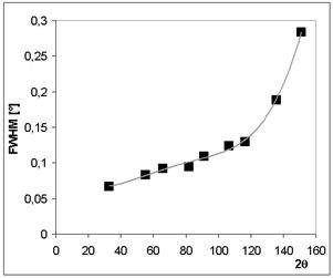
Figure 1. The FWHM vs. 2θ for CaF2 standard measured on Brag-Brentano geometry, divergent beam, soller slits, no monochromators, Co radiation, X´Celerator – detector.
The
wavelength distribution
The knowledge of the exact shape of the
source emission profile is very important in description of line profiles. In the absence of instrumental, sample and microstructural
effects it represent the highest possible resolution. Earlier it was described as two Lorentzian curves having different half-widths [9,10], but it is not relevant from the physical point of view and not compatible with the observed spectral distributions. More
detailed phenomenological representation of the Cu Kα emission profile was
first published by Berger [11]. For Cr, Mn, Fe, Co, Ni and Cu the phenomenological representations
are used to accurately represent the emission profiles from these elements with
up to seven Lorentzians being used in some cases [12].
Geometric
instrument aberrations
The most important instrument, sample, and microstructure effects contributing to powder diffraction line profiles are in Tab. 1.
Table 1. The division of effects contributing to powder diffraction line profiles [5] .
|
|
Equatorial |
Axial |
|
Instrument |
- Target width - Divergence slit angle - Receiving slit angle |
- Soller slits - Target length - Receiving slit length |
|
Sample |
- Absorption - Sample thickness - Tilt |
- Sample length |
|
Microstructure |
- Crystallite size - Microstrain - Strain - Stacking faults |
|
Divergent
beam laboratory diffractometers
The diffraction in the conventional divergent beam laboratory diffractometers is symmetric and the principal geometric aberrations contributing to a profile are i. the finite width of the x-ray source, ii. flat specimen error, iii. finite width of receiving slits, iv. specimen transparency, and v. axial divergence. Primary and secondary monochromators significantly change the emission profile.
Parallel beam diffractometers
In laboratory diffractometers is the parallel beam generated by parabolic graded multilayer mirror (Göbel mirror). The beam is parallel only in equatorial plane and not in axial, so the axial divergence is present in both incident and diffracted beam. The parallelity in diffracted beam is ensured by parallel plate collimator and/or analyzer crystals and/or channel cut monochromators. There are only two main active geometric aberrations – axial divergence and finite angular acceptance of the receiving optics. Göbel mirrors and others monocrystals significantly change the emission profile of source.
Conclusions
The computation of instrumental function instead of using measured one on the standards sample brings following advantages: The standard sample is never perfect, for example grain size should be enough large to do not cause broadening and withal not to big to product continual diffraction rings. The is another problem, that often is not available standard from the same material as the sample is, what brings problem with different absorption. Next problems may be with surface roughness and packing density.
References
1. P. Scardi and M. Leoni, Acta Cryst., A58, (2002), 190.
2.
R. W. Cheary and A.Coelho, J. Appl. Cryst., 25, (1992), 109.
3. R. W. Cheary and A.Coelho, J. Appl. Cryst., 31, (1998), 851.
4. R. W. Cheary and A.Coelho, J. Appl. Cryst., 31, (1998), 862.
5. A. Kern, A. A. Coleho, R.W: Cheary, in Diffraction Analysis of the Microstructure of Materials, edited by E.J. Mittemeijer & P. Scardi (Berlin: Springer), 2004, pp. 17-50.
6. A.J.C. Wilson, Mathematical Theory of X-ray powder Diffractometry, Philips Technical Library. 1963.
7. H.P. Klug, L.E. Alexander, X-Ray Diffraction Procedures, Wiley: New York. 1974, 2nd ed..
8. M. Čerňanský, in Defect and Microstructure Analysis by diffraction, edited by R.B. Snyder, J. Fiala, H. J. Bunge (New York: Oxford University Press), 1999, pp. 611-651.
9. J. Ladell, W. Parrish and J. Taylor, Acta Crystallogr., 12, (1959), 561.
10. J. Finster, G. Leonhardt and A. Meisel, J. Phys. (Paris)Colloq., 32, C4, (1971), 218.
11. H. Berger, X-ray Spectometry,
15, (1986), 241.
12. G. Holzer, M. Fritsch, M. Deutsch, J.
Hartwig, and E. Forster, Phys rev. A, 56, (1997), 4554.
Acknowledgements.
The research was supported by the project No: 106/07/0805 of the Czech Science Foundation.