MStruct software basic example - How to install and run.
Contents
- Installation
- Example 1: Stress Evaluation in a Thin Film Sample
Installation
The program has no GUI at present time. It runs in a command line. Text editor and an external plotting utility are required. To install program (under Windows) you may need to:
- Download and unzip the program and additional files.
- Configure your text editor to display program input parameters file tidily.
(syntax highlighting of C++ type and an 8 spaced Tab width are recommended) - Find some plotting utility for data in a multiple column text format.
The 1st step - Download and Unzip
Folder with the program should contain at least these files:
- mstruct.exe - the program itself
- libfftw3-3.dll - a dynamic library FFTW3 used for the fast Fourier transform
(Can be missing on your system and hence it is distributed with the program.) - structures.xml - few structures stored in the FOX xml file format
- LICENSE, FOX.LICENSE, README - files with license and contact information.
The folder can contain some additional files - some scripts and example files, which will be described later.
You can try double-click the mstruct.exe file now. You should see a console running, asking you for a job type.
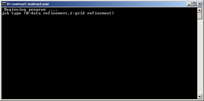 |
| The MStruct program running in a console, waiting for your answer. Write "0" for data-refinement and press "ENTER". |
The 2nd step - Setup Text Editor
The program is running in a console window without GUI. It is prompting you questions about calculation options, waiting for your response. After all program's questions are answered, the program executes a calculation. The program usually prompts you for hundreds of questions and its impossible for human being to answer them all. It is a good idea to prepare your answers in a text file and redirect the console input from this text file. You need a simple text editor to edit such a file. It is recommended to use an editor with syntax highlighting to see the input file in a pretty format. There are many suitable text editors for Windows. Free editor called PSPad can be a good choice.
The example file tio2-film-stress1.imp is an input parameter file for the first tutorial showing evaluation of residual stress
in a thin TiO2 film from a single 2Theta scan with a constant incidence angle. You can find this file in the downloaded archive together with
the program.
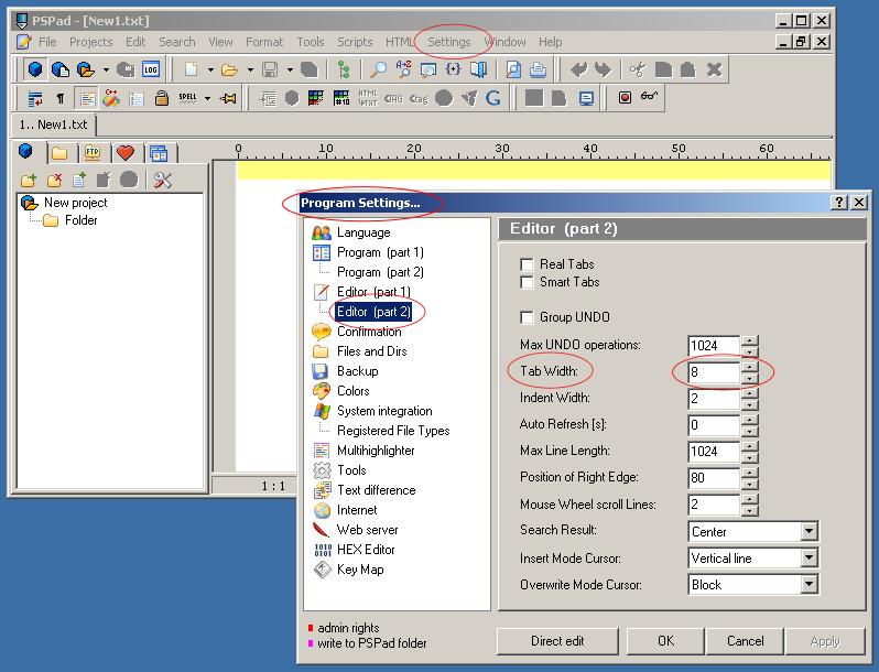
To display this file in a pretty format it is recommended to set a tab width in your editor to be equivalent to 8 spaces
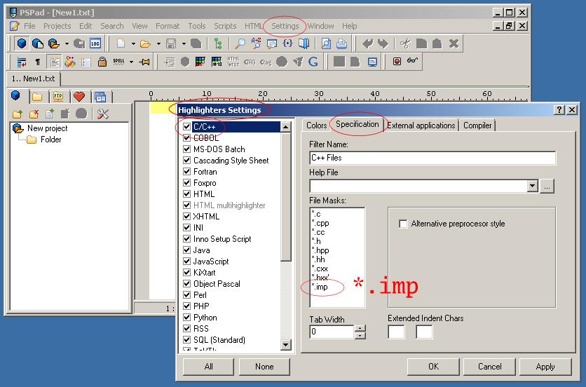
and switch on syntax highlighting settings for *.imp files to be a C++ type.
To use the program you of course need known nothing about C++. Enabled syntax highlighting should just
make orientation in the input parameters file easier (numbers and comments have different color than normal text).
 |
|
| PSPad - Tab Width Settings | PSPad - C++ Highlighter Settings for *.imp files |
When you open the tio2-film-stress1.imp input parameter file you should see properly formatted text.
If you see the input parameter file for the first time, you may see many words and numbers making no sense. This is OK. But you should no see randomly scattered words and numbers! Tab width and syntax highlighting setup is not obligatory installation step.
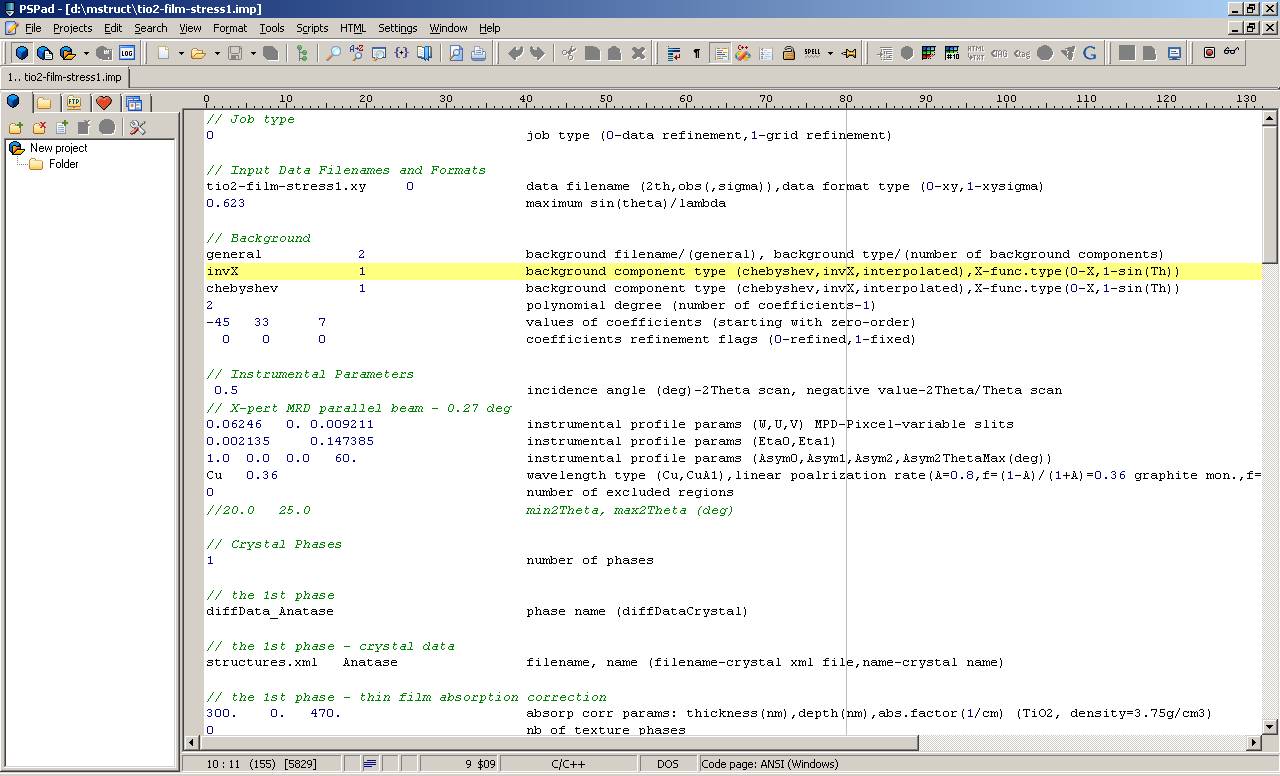 |
| PSPad - Opened tio2-film-stress1.imp input file in formatted text format with syntax highlighting |
The 3rd step - Plotting Utility
Powder pattern refinement in the mstruct program produces output data file in a column text format. Typical data output
file contains in the 1st column (2Theta) values in degrees; in the 2nd column observed intensity (Iobs),
in the 3rd calculated intensity (Icalc) and in the 4th differences (Iobs-Icalc) are printed.
| # | 2Theta/TOF | Iobs | Icalc | Iobs-Icalc | Weight | Comp0 |
| 15.0250 | 120.0000 | 111.3516 | 8.6484 | 0.0083 | 7.6486 | |
| 15.0750 | 123.0000 | 110.8423 | 12.1577 | 0.0081 | 7.6234 | |
| 15.1250 | 120.0000 | 110.3364 | 9.6636 | 0.0083 | 7.5983 | |
| 15.1750 | 120.0000 | 109.8340 | 10.1660 | 0.0083 | 7.5735 | |
| 15.2250 | 107.0000 | 109.3351 | -2.3351 | 0.0093 | 7.5487 | |
| … |
You need an utility for plotting data in this format to examine visually result of the fit or simualtion. Various sophisticated programs
can be used. You can use such tools as a free GNUPlot system, commercial expensive Matlab or you can make yourself
a smart Excel worksheet. Very simple GNUPlot
and Matlab/Octave scripts are provided with the program.
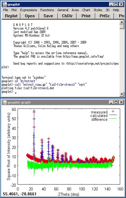
An example of how to plot data by GNUPlot or in Matlab and Octave is shown here.
Plotting data in GNUPlotThe simplest way how to use the GNUPlot program for plotting data in Windows is to:
|
Plotting data in Matlab and OctaveFor plotting data in Matlab or its free alternative - Octave (from version 3.2) - you can use Zdeněk's Matlab scripts. Download and unpack them in the program directory. There are few files:
With Matlab follow these steps:
If you are plotting data in the Matlab/Octave environment, it is useful to start program calculation directly from Matlab command line. You can use either a mstructcommand preceded with an exclamation mark ("!...") or function system(...) as: (in a single line) >> !mstruct < tio2-film-stress1.imp > tio2-film-stress1.out >> system('mstruct < tio2-film-stress1.imp >
tio2-film-stress1.out')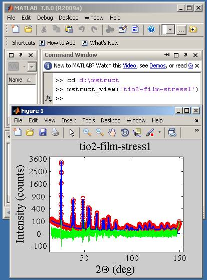
|
Example 1 - Stress evaluation in a thin film sample
This example describes residual stress evaluation in a thin TiO2 film. It illustrates how the program is used. The film is a single phase (anatase), crystallites are large (bigger than 150 nm) and there is only small microstrain in the sample (e ~ 0.2%). The sample is only slightly textured. The most interesting attribute of the sample from the XRD analysis point of view is a possible residual stress in the film. The measurement was done in parallel beam geometry with Cu-Alpha radiation as a 2Theta scan with a constant incidence angle Omega = 0.5 deg. The 2Theta angular resolution for this experiment was about 0.3 deg. For peak position corrections two effects are included:
- correction for the refraction effect at the vacuum-film interface,
- peak position correction due to simple bi-axial residual stress state in the film.
The program runs in a command line. The program prompts user for questions about calculation details and parameters. The program prints various type of information and the resulted values of fitted parameters at the end of the refinement. It is useful to store the calculation parameters in an input file (tio2-film-stress1.imp) and to catch the program text output into an output text file, which can be later checked. You can run the program from the command line in a program working directory (D:\mstruct here) by a command using input ('<') and output ('>') redirection:
mstruct < tio2-film-stress1.imp > tio2-film-stress1.out
! mstruct < tio2-film-stress1.imp > tio2-film-stress1.out
system('mstruct < tio2-film-stress1.imp > tio2-film-stress1.out')This is an example of the part of the input parameters file (tio2-film-stress1.imp):
// Job type
0					job type (0-data refinement,1-grid refinement)

// Input Data Filenames and Formats
tio2-film-stress1.xy     0		data filename (2th,obs(,sigma)),data format type (0-xy,1-xysigma)
0.623     				maximum sin(theta)/lambda

// Background
general		   2			background filename/(general), background type/(number of background components)
invX		   1			background component type (chebyshev,invX,interpolated),X-func.type(0-X,1-sin(Th))
chebyshev	   1			background component type (chebyshev,invX,interpolated),X-func.type(0-X,1-sin(Th))
2					polynomial degree (number of coefficients-1)
-45   33      7				values of coefficients (starting with zero-order)
  0    0      0				coefficients refinement flags (0-refined,1-fixed)
…
This is an example of some parts of the output parametrs file (tio2-film-stress1.out):
 Beginning program ....
job type (0-data refinement,1-grid refinement)
data filename (2th,obs(,sigma)),data format type (0-xy,1-xysigma)
maximum sin(theta)/lambda
background filename (2th,bkg),background type (0-linear,1-cubic spline)
…
finished cycle #10/10. Rw=0.22525288164616->0.22525644302368
Results after last refinement :(35 non-fixed parameters)
R-factor  : 0.07420510798693
Rw-factor : 0.22525644302368
Chi-Square: 5756.30273437500000
GOF       : 1.46968150138855
Variable information : Initial, last cycle , current values and sigma
Scale_bkgData_InvX                  20.00000000       20.80443192       20.80817223        0.10634584
Scale_diffData_Anatase               0.00000430        0.00000432        0.00000432        0.00000003
Background_Coef_0                  -45.00000000      -44.96256256      -44.95737839        0.22215381
Background_Coef_1                   33.00000000       32.32260513       32.31866455        0.30044675
…
You see in the input and output files some equivalent lines. It is useful to think awhile about how the program works and what it requires. At the beginning the program prompts you a question 'job type (0-data refinement,1-grid refinement)', as you can see on the picture somewhere above. You will answer '0' and than the program asks you 'data filename (2th,obs(,sigma)),data format type (0-xy,1-xysigma)', etc. … You can see these questions in the output file. They are are printed there because the program text output was redirected (by '>') to the file. The input file should theoretically contain only prepared answers. But it contains more! It is because:
- Empty lines, tabs and multiple spaces are ignored.
- Lines beginning with '//' are comments and are ignored.
- You can add a comment to lines with parameters/options (as you can see usually the appropriate program question is rewritten there). This comes as inspiration from old Fortran's programs. The program simply reads all parameters needed (e.g. if it prompts for two numbers, it reads two numbers) and ignores a rest of the line.
Using comments, blank spaces and line-comments you can format the input file in more clear form.
Brief description of input parameters file
Job type
// Job type
0					job type (0-data refinement,1-grid refinement)
- 0 … simple refinement of a single powder pattern
- 1 … so called grid refinement of a single powder pattern - user is later asked for a 'grid' parameter.
Refinement is always performed for each value from a set/range of user defined values of the 'grid' parameter.
- …
- > 10 … option for special jobs (pole figure simulation, etc.), jobs for development, …
Measured Data file
// Input Data Filenames and Formats
tio2-film-stress1.xy     0		data filename (2th,obs(,sigma)),data format type (0-xy,1-xysigma)
0.623     				maximum sin(theta)/lambda
- the 1st line: 2 arguments — a measured data file name and a flag for data format
(0 … 2 columns data
- 2Theta values and measured intensities in counts, or 1 … 3 columns data with weights in the 3rd column.)
- the 2nd line: value of max sin(Theta)/Lambda to which the pattern will be calculated (Lambda in A). A special word
default instead of value 0.623
can be used when whole measured pattern should be used.
// Job type 0 job type (0-data refinement,1-grid refinement)
// Input Data Filenames and Formats tio2-film-stress1.xy 0 data filename (2th,obs(,sigma)),data format type (0-xy,1-xysigma) 0.623 maximum sin(theta)/lambda
Two columns data file with experimental data should look like:
     15.0250           120
     15.0750           123
     15.1250           120
     15.1750           120
     …
Background
// Background
general		   2			background filename/(general), background type/(number of background components)
invX		   1			background component type (chebyshev,invX,interpolated),X-func.type(0-X,1-sin(Th))
chebyshev	   1			background component type (chebyshev,invX,interpolated),X-func.type(0-X,1-sin(Th))
2					polynomial degree (number of coefficients-1)
-45   30     10				values of coefficients (starting with zero-order)
  0    0      0				coefficients refinement flags (0-refined,1-fixed)
- the 1st line — code-word general saying that a genaral type background will be used and next parametr is the number of background components (2)
- the next line — type of the background component - here the invX type states that the background defined as 1/X will be used, where X depends on the second parameter. For the second parametr 0 … X(i)=2Theta(i) and for 1 … X(i)=sin(Theta(i))
- the next line — it defines the second background component and the first argument specifies the background component type to be chebyshev polynomial background. The X argument of the Chebyshev polynomial function depends on the second parameter: 0 … X(i)=(2Theta(i)-2ThetaCenter)/2ThetaRange, or 1 … X(i)=sin(Theta(i))
- the next line is also related to the chebyshev polynomial background and user is prompted for the degree of the polynomial used (here 2). The number of polynomial coeficients will be one more than the polynomial degree.
- the next line specifies the values of the backgound coeficients (one more than the polyn. degree - this means 3 values here). The first coeficient is the zero order polynomial coeficient etc.
- the last line specifies for each of polynomial coeficient its state during refinement: 0 … not fixed=refined, or 1 … fixed
Instrumental function
// Instrumental Parameters
 0.5					incidence angle (deg)-2Theta scan, negative value-2Theta/Theta scan
// X-pert MRD parallel beam - 0.27 deg
0.06246   0. 0.009211   		instrumental profile params (W,U,V) MPD-Pixcel-variable slits
0.002135     0.147385       		instrumental profile params (Eta0,Eta1)
1.0  0.0  0.0   60.			instrumental profile params (Asym0,Asym1,Asym2,Asym2ThetaMax(deg))
Cu   0.111				wavelength type (Cu,CuA1),linear polarization rate(f),
//                                      (A=0.8,f=(1-A)/(1+A)=0.111 graphite mon.,f=0. unmonochromatized)
0					number of excluded regions
//20.0   25.0				min2Theta, max2Theta (deg)
- The incidence angle value is also used to specify the diffraction geometry used. It is essential for correct intensity correction and residual stress evaluation. A value higher than zero specifies parallel beam geometry with the given incidence angle. Values less than zero (e.g. -1.0) are used for the Bragg-Brentano case and negative values less than ~-1.99 (e.g. -2.0) should be used for the Bragg-Brentano geometry with variable slits.
- A phenomenological pseudo-Voigt function is used to describe the instrumental broadening. A standard sample should be
measured in the same experimental arrangement and the angular dependence of FWHM, Gauss/Cauchy ratio and asymmetry
of the standard sample peaks fitted by the pseudo-Voigt functon should be approximated by polynomials. Polynomial
coefficients can than be used to describe the instrumental broadening function here.
- FWHM(deg)^2 = U * tan(Th)^2 + V * tan(Th) + W
(where FWHM is a parameter-FWHM, not true-FWHM in the case of asymmetrical profiles) - Eta = Eta0 + Eta1 * 2Th(rad)
(0…pure Gaussian peak, 1…pure Lorentzian) - Asym = Asym0 + Asym1 / sin(2Th) + Asym2 / sin(2Th)^2 for 2Th(deg) < Asym2ThetaMax(deg) else Asym = 1 (symmetrical peak)
- FWHM(deg)^2 = U * tan(Th)^2 + V * tan(Th) + W
- The radiation is specified by a code-word Cu indicating copper tube and K-alpha1 - K-alpha2 doublet. Next to the radiation polarization rate f is set. f=0 means unmonochromatised radiation. A = cos(Th_mono) parameter is often used instead of f to specify the monochromator in some programs. The polarization ratio can be calculated from the A parameter as f = (1-A)/(1+A). In the case of a graphite monochromator A=0.8 and f=0.111.
Crystal and Diffraction data
Here we become to more crystallographic parts of the problem.
// Crystal Phases
1					number of phases

// the 1st phase
diffData_Anatase			phase name (diffDataCrystal)

// the 1st phase - crystal data
structures.xml   Anatase		filename, name (filename-crystal xml file,name-crystal name)
- User is prompted for a number of crystal phases in the sample.
A section for each crystal phase follows with :
- a crystal phase name — It is convenient in the original FOX program to give a name to each object. These names for user objects (Crystals, Peak broaedening effects, etc.) are very useful in MStruct because they can be later used to adress model parameters. Here a crystal phase called "diffData_Anatase" is defined.
- crystal structure of new crystal phase is read from an user defined crystal structures database file. Its name is
"structures.xml" here and a crystal with name "Anatase" is loaded from the file.
The "structures.xml" file is an xml file containing definitions of several crystal structures in the FOX/ObjCryst xml format. A simple way how to create a new structure and add it into the database file is to use the original FOX program to create the Crystal structure, save the Crystal in the standard FOX xml format and using a text editor copy/paste the Crystal into the database file. (example of an xml file defining anatase crystal structure)
Thin film absorption correction
// the 1st phase - thin film absorption correction
300.    0.   470.			absorp corr params:thickness(nm),depth(nm),abs.factor(1/cm) (TiO2,dens=3.75g/cm3)
0					nb of texture phases
1	1				hkl file(0-don't use,1-generate,2-free all,3-read),print HKLIntensities(0-no,1-y)
- the 1st line — absorption correction parameters: a film thickness in (nm), a depth (nm)
- distance from a sample surface and an absorption factor - µ (1/cm) are specified. If you would like to
specify a bulk sample, set the thickness to be a negative value and the depth equal to zero. You can use e.g.
Sergey Stepanov's chi0 pages to calculate absorption coefficient
for the material of your interest.
The intensity corrections is calculated according to:If (T >= 0) : Iabsorp = Tp/sin(ω) (1 - exp(-T/Tp)) exp(-D/Tp),
and a penetration depth is calculated from 1/Tp = μ ( 1/sin(ω) + 1/(sin(2Θ-ω) ),
If (T < 0) : Iabsorp = 1/(2μ),
where T is the film thickness, D is the depth (effective distance of the scattering layer from the sample surface), μ is the absorption coefficient and ω is the incidence angle.- Note: The same penetration depth is used for a thin film intensity contribution as for the absorption correction in the above layered structure. In case of materials with different absorption the depth parameter D has to be recalculated so the (μD) factor is kept constant.
- Note: To current knowledge the above absorption correction is not correct in some cases, especially close to the angle of the total external reflection.
- D.Simek, R.Kuzel, D.Rafaja, J.Appl.Cryst(2006) 39, 487-501
- T.Noma, A.Iida, J.Synch.Rad.(1998), 5, 902-904
- P.Colombi, P.Zanola, E.Bontempi, L.E.Depero, Spectroch.Acta (2007) B62, 554-557
- D. Rafaja, Adv.Solid State Phys. (2001) 41, 275-286
- Z.Matej, L.Nichtova, R.Kuzel, Z. Kristallogr. Suppl. (2009) 30, 157-162
- Sergey Stepanov's X-ray Server: http://sergey.gmca.aps.anl.gov
- the 2nd line — number of additional intensity corrections. Set to zero here. In addition to standard (Lorentz, polarization, slit, absorption) intensity corrections other effects can be included - especially texture.
- the 3rd line — indicates how “reflections intensities correction” Ihkl-file is used. This option represents something like so called arbitrary texture correction (in Maud). Calculated intensity of each reflection can be multiplied by an arbitrary value. This value can be either set fixed or refined. How the Ihkl file is used will be described later in detail. Here the choice is set to 1, which means that the Ihkl file "Ihkl_diffData_Anatase.dat" will be generated. Please note how the file name and the diffracting phase name "diffData_Anatase" are related. The second choice (here 1) specifies that the reflection intensities correction factors should be printed at the end of the refinement.
Micro-structural effects - Size broadening
// the 1st phase - physical line broadening
4					number of additional effects

// the 1st phase - Size broadening - lognormal distribution of crystals diameter (median - M, shape - Sigma)
SizeLn	       sizeProfAnatase		broadening component type (pVoigt(A),SizeLn,dislocSLvB,HKLpVoigtA),effect name
200.0     0.3				M(nm),sigma
- Number of effects causing peaks broadening, shift, etc. is given here. After this point the program will wait for a type-name, an object-name and specific parameters for each effect.
- Size broadening effect described by spherical crystallites and the log-normal distribution of their diameter (D)
is set by the code word SizeLn. This size broadening effect for the anatase crystal
phase is named "sizeProfAnatase" by the second argument at the line. This profile broadening component is convoluted
with the instrumental broadening specified above and all others broadening effects. The model is described in e.g these
original references:
- G.Ribarik, T.Ungar, J.Gubicza, J.Appl.Cryst.(2001) 34, 669-676: MWP-fit
- P.Scardi, M.Leoni, ActaCryst.(2002) A58, 190-200
- Lognormal distribution: p(D) = 1/(sqrt(2*pi)*σD) exp( (ln(D/M))² / (2σ²) ),
see also: E.Limpert, W.A.Stahel, M.Abbt, Log-normal Distributions across the Sciences: Keys and Clues, May (2001) / Vol. 51 No. 5, BioScience, 341-352
- At the last line the median of the diameter distribution M and the "shape" parameter σ of the log-normal distribution are set.
In some conventional definitions of the log-normal distribution M = exp(μ) (→MathWordl).
Micro-structural effects - Microstrain broadening
// the 1st phase - Strain broadening - simulated with pseudoVoigt function
//                                   - only U-Cagliotu param. (W=V=0.) and shape Eta0 (Eta1=0) params. refined
pVoigtA	       strainProfAnatase	broadening component type (pVoigt(A),SizeLn,dislocSLvB,HKLpVoigtA),effect name
0.0  0.  0.				profile params (W,U,V)
0.0       0.				profile params (Eta0,Eta1)
1.   0.   0.   60.			profile params (Asym0,Asym1,Asym2,Asym2ThetaMax(deg))
- Another profile broadening component is a microstrain effect. The effect is described here phenomenologically by a pseudo-Voigt function. Its width is calculated from the Caglioti polynomial with only U coefficient nonzero. The code-word for the pseudo-Voigt function is pVoigt. However it is usually more convenient to convolute broadening effects in the Fourier space and this is used here by an appropriate code-word pVoigtA. The second argument at the line is a name used for this effect for the anatase crystal phase: "strainProfAnatase".
- W, U, V coefficients of Caglioti polynomial. W, V are zero by definition of the model. U is set zero, because a zero microstrain is assumed here.
- Eta0 and Eta1 coefficients for the shape parameter. The model assumes 2Θ independent profile shape. Hence Eta1 is fixed to zero and the reflection profile shape connected with the microstrain effect is given by the Eta0 value: 0…Gaussian , 1…Lorentzian.
- Asymmetry parameters — Profile is assumed to be symmetric in a whole 2Θ range. Hence Asym0 is equal to 1 and other coefficients are zero.
- The Fourier/direct space pseudo-Voigt function used here for description of the microstrain broadening effect is a weighted sum of
the Fourier transform of the Gauss and Caychy functions (ref. Scardi (1999)):
pVoigtA(x) = (1-k) exp(-π² σ² x² / ln2) + k exp(-2π σ |x|),
1/k = 1 + (φC/φG) (1-η)/η , φG=2sqrt(ln2/π), φC = 2/π,
x … is a direct/real space variable.
This means that the reciprocal space (s=1/d) pseudo-Voigt function is defined as:IFT( pVoigtA )(s=1/d) = (1-η) exp(-ln2 (s/σ)²) + η 1/(1+(s/σ)²),
σ = FWHM/2
and hence the pseudo-Voigt function used here is different from the convenient (e.g. in FOX/ObjCryst) pseudo-Voigt function, which is usually defined to be a sum of normalised Gauss and Cauchy functions in the reciprocal space units (s=1/d) with weights (1-η) and η respectively. (η is the symbol for the parameter Eta here)- B.E.Warren, X-Ray Diffraction, Addison-Wesley, Reading, MA (1969)
- P.Scardi, M.Leoni, J.Appl.Cryst.(1999) 32, 671-682
- The microstrain effect is usually assumed to produce Gauss-like peak broadening. Here the shape of the broadening
component can be varied by a choice of the Eta0 parameter. Then from the U
and Eta0(=η) parameters the microstrain e can be calculated from:
FWHM(2Θ[rad])² = U tan²(Θ), β(2Θ[rad]) = 4e tan(Θ),
4e = ((1-η)/φG + η/φC) sqrt(U)
(φG and φC are defined above) - Some details can be found also in: Z.Matěj, R.Kužel, L.Nichtová, Powder Diffraction (2010), 25(2), 125-131
Micro-structural effects - Refraction correction
// the 1st phase - Refraction reflection position correction
RefractionCorr   refractionCorrAnatase  effect type,effect name
crystal					chi0 set directly-value,calc from-crystal,calc from chem.-formula
1.					relative density
- A little uncommon effect included here is the refraction correction (codeword
RefractionCorr). Next at the line a phase specific name for the effect
“refractionCorrAnatase” is also given.
A thin film sample is measured in the parallel beam geometry with a low incidence angle. Even thought the refraction index of the film is only slightly less than one, refraction of x-rays on the the air(vacuum)-film interface can not be neglected for incidence angles which are close to the critical angle of a total external reflection. The incidence angle is 0.5° and the critical angle for a TiO2 film α_c is approx. 0.27°. The effect causes a constant shift of all reflections about 0.09° in this case. It can be simulated by a “2Theta zero shift”, but with two shortcomings: 1) The “zero shift” is unrealistically large and depends on the incidence angle. 2) The trick does not work for multilayered structures with different electron density of diffracting layers. - A complex dielectric susceptibility chi0 is required for calculation of the effect. It can be derived from the crystal structure. This is done by using the codeword crystal at the 2nd line. Other options are to calculate the susceptibility from the chemical formula and material density, or set it directly by using the codeword value. Regardless of how the susceptibility was set it will be considered as a reference structural susceptibility and called chi0_struct in the next step.
- The only parameter of the model - relative density (n_r) - is specified at the last line. If a real density
of the film is different from that calculated/prescribed, the susceptibility of the film chi0_film can also be
calculated as a product of this factor and the structural susceptibility chi0_struct
chi0_film = n_r * chi0_struct .
There is also a simple relation between the susceptibility and the critical angle α_calpha_c = sqrt |chi0| .
This gives for a real (porous) sample a relation between the critical angle α_c(struct) calculated from chi0_struct, critical angle α_c(exp) measured e.g. by x-ray reflectivity and the relative densityn_r = [α_c(exp)/α_c(struct)]^2 .
Note: A simple manual how to set the correct value n_r may be: 1) measure the critical angle α_c(exp) of the film by x-ray reflectivity, 2) let MStruct calculate the structural α_c(struct) (see below) and 3) set n_r according to the equation above.
Note: MStruct during its run shows some relevant information. For example, when refraction correction effect is included and susceptibility chi0 is calculated from the crystal structure, program prints also the value of a critical angle α_c(struct).Hence you can let run the program once with n_r = 1 and then in the second run use the value printed by the program and the guideline above to set the correct value.… MStruct::RefractionPositionCorr::GetChi0(...): Chi0 and absolute density computed for Crystal: Anatase chi0: (-2.3988e-05,-1.2128e-06) (n=1-delata-ii*beta~=1+chi0/2) critical angle: 0.28(deg) density: 3.891 (g/cm3) …
Note: If you prefer to set the susceptibility chi0 by value, Sergey Stepanov's X-ray Server can be a valuable tool for you. - The effect of refraction on powder diffraction line positions was already described by Hart (1988) and also some time ago
e.g. by Colombi et al. Some references can be found below.
- M. Hart, W. Parrish, M. Bellotto, G.S. Lim, Acta Cryst. (1988) A44, 193-197
- F. Toney, S. Brennan, Phys.Rev.B (1989) 39, 7963-7966
- P. Colombi, P. Zanola, E. Bontempi, R. Roberti, M. Gelfib, L.E. Depero, J.Appl.Cryst. (2006) 39, 176-179
- D. Rafaja, Adv.Solid State Phys. (2001) 41, 275-286
- S. Wronski, K. Wierzbanowski, A. Baczmanski, A. Lodini, Ch. Braham, W. Seiler, Powder Diffraction (2009), 24(S1), 11-15
- Z. Matěj, R. Kužel, L. Nichtová, Powder Diffraction (2010), 25(2), 125-131
- D. Simeone, G. Baldinozzi, D. Gosset, G. Zalczer, J.-F. Bérar, J.Appl.Cryst. (2011) 44, 1205-1210
- Sergey Stepanov's X-ray Server: http://sergey.gmca.aps.anl.gov
Micro-structural effects - Residual stress effect
// the 1st phase - Residual stress reflection position correction - simple stress model
StressSimple   stressCorrAnatase  	effect type,effect name
Reuss-Voigt     0.			XECs model, stress (GPa)
// material C11 C12 C13 C33 C44 C66 constants (in GPa) - in the format: C11 value C12 value etc.
C11 320  C12 151  C13 143 		// anatase Cij (GPa)
C33 190  C44  54  C66  60		// ref: M.Iuga,Eur.Phys.J.B(2007)58,127-133
0.3					model weight (0..Reuss,1..Voigt)
- The last and the most interesting effect included here is a residual stress correction. A codeword for the effect is StressSimple. Next at the first line the effect is also given a phase specific name.
- The StressSimple model assumes a very simple homogenous bi-axial stress state in the film characterised
by a single stress value (σ). Then we can write for strain
ε(hkl,ψ) = 1/2 S_2(hkl)*σ sin²(ψ) + 2 S_1(hkl)*σ ,
where ψ is the inclination angle of diffracting planes normals from the sample surface normal and S_1 and S_2 are x-ray elastic constants (XECs). - The film is a polycrystalline aggregate and a relation between the residual stress state in the sample and the strain in crystallites has to be considered within the grain interaction model to derive XECs. The program prompts for this model at the 2nd line. You can specify either an isotropic model. Then Young's modulus and Poisson's ratio for the film are required at the next line. Alternatively a weighted combination of Reuss and Voigt models can be set by a codeword Reuss-Voigt. Next at the 2nd line the stress value (σ) is set to zero. It is together with the choice of XECs model, the only intrinsic parameter of the StressSimple model.
- Next section describes parameters of the Reuss-Voigt XECs model. Within the StressSimple and the Reuss
model XECs are hkl-dependent. Fortunately XECs can be calculated from single crystal elastic constants (Cij) if they
are known (see references of Popa and Hauk). Hence MStruct prompts for single crystal elastic constants for a particular
phase. The stiffness constants should be entered in a form:
The spaces and the order of Cij constants are not important. Only constants required by crystal symmetry should be entered. Program prints their list. The constants can be set on multiple lines, which is usually not allowed in the program. The units are Giga Pascals here, but actually they are the same as that for the stress value. Elastic constants for anatase from a reference in comments - Iuga (2007) - are taken here. Program prints information about the entered values.
  C11 value C12 value …
  C11 320  C12 151  C13 143 …
  Stiffness constants:
	C11: 320 (GPa)
	C12: 151 (GPa)
	C13: 143 (GPa)
	C33: 190 (GPa)
	C44: 54 (GPa)
	C66: 60 (GPa)
  Stiffness tensor in the Voigt notation (GPa):
	       320       151       143         0         0         0
	       151       320       143         0         0         0
	       143       143       190         0         0         0
	         0         0         0        54         0         0
	         0         0         0         0        54         0
	         0         0         0         0         0        60
- At the last line a Reuss-Voigt model weight factor (w) is set. XECs for the bounding models Voigt - S_i(Voigt)
and Reuss - S_i(hkl,Reuss) are calculated. Their weighted average is then substituted in the equation for strain.
S_i(hkl) = w * S_i(Voigt) + (1-w) * S_i(hkl,Reuss) , i = 1, 2
- Some useful references can be:
- H. Behnken, V. Hauk, Z.Metallkd. (Int.J.Mater.Res.) (1986), 77, 620–26.
- N.C. Popa, J.Appl.Cryst. (2000), 33, 103-107
- U. Welzel, J. Ligot, P. Lamparter, A.C. Vermeulen, E.J. Mittemeijer, J.Appl.Cryst. (2005), 38, 1-29
- D. Rafaja, Adv.Solid State Phys. (2001) 41, 275-286
- M. Dopita, D. Rafaja, Z. Kristallogr. Suppl. (2006), 23, 67-72
- Z. Matěj, R. Kužel, L. Nichtová, Powder Diffraction (2010), 25(2), 125-131
- Z. Matěj, R. Kužel, L. Nichtová, Metal. Materials Trans. A (2011), 42, 3323-3332
After a wide section including all various physical effects affecting width, shape and position of diffraction maximas there are two sections. One setting output data file and the another one specifying refinement parameters. For most of the refinement procedure the user need to modify especially this last part.
Output file name
// output filename
tio2-film-stress1.dat output filename- The output data file is specified here. Data are saved in a multicolumn format described in the Plotting utility part.
Refinement parameters
// number of refinement iteractions
15					nb of interactions
// number of parameter which will be set
14					nb of params
This is the first part of the refinement parameters section.
- A number of LSQ refinement steps is set at the 1st line. The Levenberg-Marquardt algorithm is used. If the number is zero here, no iterations are done and data are only simulated. If the number of iterations is positive, refinement procedure will be stopped either after some convergence criteria are achieved or after maximum steps equal to this number. If the number is negative, convergence criteria are ignored and exactly the specified (of course positive) number of iterations are done.
- The value at the 2nd line sets a number of parameters, that are to be set in the next section.
Refinement parameters section
// begin of the parameters section
// *********************************************************************************

Scale_diffData_Anatase   		* param name
1.e-6					scale
4.0  0.01				value, derivative step
0					limited (0,1), min, max
sizeProfAnatase:M			* param name
10.					scale
270.0       2.0              		value, derivative step
1 2. 500.				limited (0,1), min, max
Two parts above show two typical sections of the last part of the input parameter file, where actual values and refinement flags for parameters are finally set.
PARAMETERNAME				* param name
SCALE					scale
VALUE  DERIVSTEP			value, derivative step
LIMITED  MIN  MAX			limited (0,1), min, max
A section for each parameter has 4 lines.
- The parameter name is at the 1st line.
In the second example above, where a median (M) of the log-normal size distribution of anatase crystallites is set (sizeProfAnatase:M). You can recall a fragment of code in the input file above, where crystal structure was specified. There can be multiple crystallites phases using the same model and hence a parameter name “M” could be ambiguous. The same case may happen with atomic coordinates (x) etc. You can use an object specific name “sizeProfAnatase” and a single colon notation to address the parameter more closely as: sizeProfAnatase:M.
If you have no idea what are the names of parameters of your interest, let the program do a simulation, look in the program output file (out-file), before refinement the program prints a list of all parameters. This is a feature of the original Fox.
#0#Zero:                0.000000000000 Fixed
#1#2ThetaDispl:         0.000000000000 Fixed
#2#2ThetaTransp:        0.000000000000 Fixed
#3#DIFC:            48277.140625000000 Fixed
#4#DIFA:               -6.699999809265 Fixed
#5#Scale_bkgData_InvX: 20.000000000000
#6#Scale_diffData_Anatase: 0.000004000000
#7#Wavelength:          1.541836619377 Fixed
#8#Background_Coef_0: -45.000000000000
#9#Background_Coef_1:  30.000000000000
#10#Background_Coef_2: 10.000000000000
#11#Global_Biso:        0.000000000000 Fixed
#12#diffData_Anatase_Ihkl_1_0_1:  1.000000000000 Fixed
#13#diffData_Anatase_Ihkl_1_0_3:  1.000000000000 Fixed
...
#95#M:    270.000000000000 Limited (2,500)
#96#Sigma:  0.300000011921 Fixed
...
#105#Density:    0.959999978542 Fixed
#106#Stress:     0.000000000000 Limited (-100,100)
#107#RV_weight:  0.300000011921 Fixed
- A program to human scaling factor is specified at the 2nd line. The scale factor for the intensity parameter of anatase phase (Scale_diffData_Anatase) has just a practical reason that you don't need write ugly numerical values later. However the scale factor for the sizeProfAnatase:M parameter above, equal to 10.0 here, has some meaning. Program performs all calculations in Angstroms, which are useful measures of lattice parameters, but crystallite size is rather measured in nanometers. The value (10.0) here converts the human “readable” units (nanometers) into the program units (Angstroms). A specific value (0.0175) can be seen within some angular parameters (2Theta Zero-shift error) further in the input file. It is simply a (π/180) ratio converting angular degrees to radians. Its square (3.0462e-4) converts a Caglioti parameter “U” from squared degrees to squared radians etc.
- A parameter actual value and its derivative step are set at the 3rd line. The program needs to calculate
derivatives with respect to refined parameters and it utilises a numerical method in most of cases. Some parameters, for example
scale factors, are exceptions. The derivative step specified here should be an appropriate positive value. For example a reasonable
choice for the “sizeProfAnatase:M” is approx. 2-10 nm if crystallites are larger than 100 nm,
but for nanoparticles of size 4.0 nm a 0.1 nm derivative step would be much more better choice.
- If the derivative step is set zero (0.0), the parameter is not refined, but before refinement it is set to the specified value. Hence you can use this section to set all parameters of your choice.
- For diffraction components scales the derivative step value is not important, but if it is zero the parameter is not refined.
- The scale ratio set above is used to convert the user specified values to program units.
- You can also set limits for the parameter if you set the first value at the 4th line to one (1). Contrary if it is set
to zero (0) then no limits are applied. For example, the size parameter “sizeProfAnatase:M”
should be a positive value and it is also unreasonable if the value is higher than e.g. 500 nm when the broadening
effect is negligible. Hence these limits are applied to the parameter as you can see that the minimum is set to 2.0 nm and
maximum 500 nm.
The Reuss-Voigt weight parameter for the residual stress model described above should be always in the range (0,1). This parameter (“stressCorrAnataseXECs:RV_weight”) can be found further in the file and you can see how the limits are set.