New empirical expressions to calculate the transmission factor for cylindrical samples

J. Birkenstock¹

¹Universitaet Bremen, FB5-Kristallographie, Klagenfurter Str.2, D-28359 Bremen, Germany.

The calculation of the intensities of reflections in diffraction experiments includes a transmission factor T which is dependent on the geometry of the diffraction experiment. While for the common Bragg Brentano reflecting geometry the transmission factor is assumed to be constant for all angles 2θ of diffraction T is a function of 2θ for transmission measurements. Among others in [1] and [2] values of T are given for cylindrical samples as a function of discrete θ and μ·R being calculated by numerical integration, where μ is the samples absorption factor and R the radius of the cylinder. Here, μ·R ranges from 0 to 20 in [1] and 0 to 2.5 in [2], with three significant digits in [1] and five in [2]. These values have been used by several authors and also here as reference data to develop simple empirical expressions to calculate T as a function of given θ and μ·R.

The expressions given in [3] have been used in Rietveld programs for many years, though it was explicitly limited to be valid up to μ·R ≤ 1 which is usually fulfilled for neutron diffraction experiments but often not for x-ray diffraction. This e.g. has been pointed out by [4] who used the following approximating formula to calculate T as a function of θ and μ·R:

(1)

where A_L and A_B are the absorption factors at the Laue and the Bragg condition, i.e. at θ = 0° and 90°, respectively. A_L and A_B can be calculated by extensive analytical expressions, cited from [5], as a function of μ·R. Using (1), the maximum deviations from the tabulated values in [1] are given at θ = 45°, ranging from 1 % for μ·R = 1 to 20 % for μ·R = 20. Thus the largest errors occur where the density of reflections is usually rather high.

A simple modification of (1) was used here yielding a different approximation of the reference data:

(2)

With this fully empirical approach the coefficients A, B, C and D can no longer be calculated directly and thus have been determined for each tabulated μ·R by the least squares method, fitting (2) to the tabulated values. This yielded for each μ·R a separate set of A, B, C and D. Fig. 1 displays the coefficients A – D as functions of μ·R.

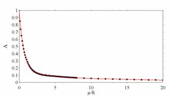
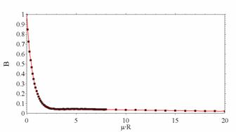
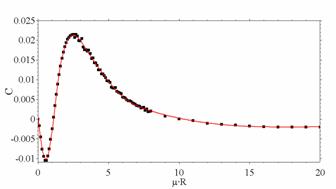
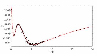
Figure 1: Solid dots are the refined coefficients A, B, C respectively D of eq. (2) as a function μ·R. The solid lines represent empirical curves calculated from equations (3) – (6) obtained by a second refinement.

The resulting errors at θ = 45° between the calculated values and the tabulated ones range from 0.06 % for μ·R = 1 to 2.4 % for μ·R = 20 and from visual inspection the overall agreement is much better than in [4]. It is noted that a more rigorous comparison could be based on residuals or Chi² values, but these are not given in [4]. In contrast to [4] the maximum deviations occur at θ = 0° ranging from 0.07 % for μ·R = 1 over 1.4 % for μ·R = 5 and 53 % for μ·R = 10 to 325 % for μ·R = 20, i.e. being rapidly increasing inaccurate with higher μ·R. At the practically more meaningful observation angle of θ = 5°, though, the deviations are much less being 0.02 % for μ·R = 1, 5.9 % for μ·R = 5, 9.6 % for μ·R = 10 and 11.6 % for μ·R = 20, respectively.

Due to the much better overall agreement of (2) with the tabulated values and the fact that the density of reflections at lower angles is usually much less than at intermediate angles (2) is considered to be preferable to (1).

From the coefficients A – D the transmission factor may be computed for any diffraction angle, but only for the discrete values of μ·R which are given in [1] and [2]. For intermediate values of μ·R interpolated values A – D have to be derived. This is non-trivial in regions where the coefficients are somewhat erratically spread with small changes of μ·R. Thus, in a second refinement step, for each coefficient A, B, C and D an individual empirical function was set up to describe it as a function of μ·R from which the respective coefficient can be calculated directly for any given μ·R. The respective functions are:

(3)

with: A_A = 0.8222(46), B_A = 0.6437(71), C_A = 0.1543(45), D_A = -0.0188(17), E_A = 0.00117(19), F_A = -2.67(59)·10^-5

(4)

with: A_B = 1.0454(87), B_B = 0.6695(54), C_B = -0.0537(92), D_B = 0.0509(57),
E_B = -0.00968(13), F_B = 0.00084(14), G_B = -3.43(69)·10^-5, H_B = 5.4(1.2)·10^-7

(5)

with (n.r. = not refined): A_C = 0.0076(29), B_C =1.60(19), C_C = 2.4142(n.r.), D_C = -0.0368(22), E_C = 1.315(34),
F_C = 0.55435(n.r.), G_C =0.0264(33), H_C = 3.34(13), I_C = 3.27(19), J_C = 0.01613(87), K_C = -0.00247(19),
L_C = 8.9(1.1)·10^-5, M_C = -1.40(47)·10^-9

(6)

with: A_D = 0.0043(46), B_D = 0.82(30), C_D = 1.932(51), D_D = -0.0215(37), E_D = 0.887(72), F_D = 0.592(21), G_D =0.0198(95),
H_D = 1.92(47), I_D =2.73(29), J_D = -0.0589(40), K_D = 0.00274(58), L_D = -4.6(2.0)·10^-5, M_D = 0.0665(55), N_D = 1.82(25)

In Fig. 1 the solid lines represent the curves that have been calculated from equations (3) to (6). Thus, in reversed order, for a given μ·R the coefficients A – D may be calculated from eqs. (3) – (6) from which T can be calculated for a given θ by eq. (2). Since the errors of some parameters are rather high compared to the values themselves it was tested if the respective terms could be omitted. But it turned out in all cases that the resulting fit is much worse both from the respective residuals and the graphical inspection. Thus the above formulas represent an operative way to calculate transmission factors for all values of μ·R ranging from 0 to 20.

[1] J.S. Kasper, K. Lonsdale (eds.), International Tables for X-ray Crystallography, Vol II (1972), Kluwer Academic Pub., Dordrecht

[2] A.J.C. Wilson (ed.), International Tables for Crystallography, Vol C (1995), Kluwer Academic Pub., Dordrecht

[3] K.D. Rouse, M.J. Cooper, Acta Cryst. A26 (1970), 682-691.

[4] T.M. Sabine, B.A. Hunter, W.R. Sabine, C.J. Ball, J. Appl. Cryst. 31 (1998), 47-51.

[5] C.W. Dwiggins, Acta Cryst. A28 (1972), 219-220.