Calculating the peak shape of axially focussing powder diffractometers

Daniel M. Többens

Hahn-Meitner-Institut, Glienicker Straße 100, D-14109 Berlin, Germany

The accurate description of the shape of individual peaks is essential for high quality Rietveld refinements. Systematic errors of the peak shape reduce the precision of the refinement and can result in parameters refined to systematically wrong values. Due to the speed of modern computers pure numerical calculation of peak shapes has become feasible. Thus instrument geometries increasing the intensity can be chosen, even if more complicated peak shapes without good analytical description result. Pure numerical Monte-Carlo simulations show good results simulating instruments. However, they still take to long to be used in routine Rietveld refinement, where relevant parameters, i.e. sample height, can vary from one measurement to the next.

In neutron powder diffraction, axially focussing monochromators have become widely used. The geometry of these instruments (see figure) results in peak shapes for which a description by currently available non-MC models is not satisfying. The peak shape is mainly determined by the instrumental axial asymmetry function (AAF). A fundamental approach for calculating the AAF for this type of geometry is discussed in this paper. The various effects to be considered are explained in detail and a programme, QUASIMODO, to do the calculations is presented.

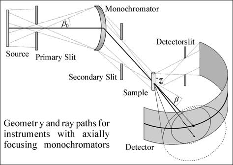
The strongest influence on the AAF results from the projection of the Debye cone on the cylindrical detector. Since the width of the detector aperture is not zero a curved section of the Debye cone is observed. The projection of this section on the cylindrical detector is in first approximation a parabola. In most discussions of the AAF this parabolic approximation is used. In the case of a shift of the Laue cone's origin along the axis of the sample (z-shift), one arm of the parabola is shortened while the other is elongated, resulting in an increased asymmetry. This effect has been discussed in detail in many publications (i.e. Finger et al [1]). In the case of a parallel primary beam, this is sufficient to describe the AAF in terms of sample height and detector height. However, it is not sufficient for the case of a converging beam discussed in this paper.

When axial divergences are considered, Debye cones will be tilted out of the main diffraction plane of the instrument (β-tilt). This affects the AAF in a way similar to the z-shift. In a geometry with an ideally focussing monochromator all rays of the primary beam hit the sample at the same point, right in the macroscopic diffraction plane. The height of the sample, otherwise an important factor for the asymmetry function, is thus effectively zero and the height of the monochromator becomes the important factor. The resulting AAF is similar, but not identical, to that resulting from the parallel beam model and its dependency on the Bragg diffraction angle is different. Moreover, the shape of the reflections is strongly dependent on the focus length of the monochromator. If the monochromator focuses directly on the sample, the diffraction peaks have very high asymmetry [2]. If the focus is behind the sample, the two effects of z-shift and β-tilt correlate in a way to cancel out each other. In order for this to be most effective, however, the sample must be high enough. In general this is not the case, thus an increase in sample height would reduce the asymmetry in most instrumental set-ups of this type.

The final AAF is determined by the distribution of the intensity in the two parameter space of sample height and axial divergence angle. For its calculation the respective heights, distances and angles of source, monochromator, sample and detector all have to be considered. Additionally, apertures between source and sample block some of the possible paths, thus changing the intensity distribution. Apertures between sample and detector block parts of the Debye cone only and therefore have to be treated differently from those in front of the sample.

An additional influence on the AAF results from the difference between the macroscopic monochromator diffraction angle 2α and the real diffraction angle 2θ_M of the Laue condition. Their relation depends on the tilt angles β₀ of the primary ray and β of the secondary ray as cos 2θ_M = cos 2α cos β₀ cos β + sin β₀ sin β. In a focussing geometry β₀ and β have opposite signs for most rays, resulting in 2α < 2θ_M.

The program QUASIMODO calculates the peak shape by means of a combination of ray tracing and analytical approach, using ray tracing in front of the sample and an analytical expression for the projection of the Debye cones. The source of rays is modelled as a linear source of limited height with isotropic emission. Each calculated ray is described by its initial height above the macroscopic diffraction plane and by its initial angle with respect to it. The way of the rays are calculated through various slits placed between the source and the monochromator and between the monochromator and the sample, respectively. For those rays hitting the monochromator the reflected ray is calculated according to the Laue equation based on the orientation of the monochromator crystals diffraction vector. Thus the resulting angles β and heights z for those rays hitting the sample are a result of the initial values at the source and the orientation of the respective monochromator crystal.

For each ray hitting the sample the AAF for a Bragg reflection with a given value of 2θ is calculated from the projection of the ray's individual Debye cone on the cylindrical detector; for this the full function is used instead of the parabolic approximation. Shifts due to deviations of 2α from 2θ_M are applied after that. The AAF of all rays are added up to give the final AAF of the reflection, which is folded with a Gaussian function in order to include the horizontal broadening. Fitting the parameters of peak width and AAF to an experimental data set is possible. Experimental tests have been done with data measured on E9 at the HMI [3].

[1] Finger, L. W.; Cox, D. E.; Jephcoat, A. P.: J. Appl. Cryst. 27, 892-900 (1994)

[2] Többens, D. M.; Tovar, M.: Applied Physics A, A74, 136-138 (2002)

[3] Többens, D. M. et al.: Mater. Sci. Forum. 378-381, 288-293 (2001)